in Empirical Microeconomics
Richard Blundell
Monica Costa Dias
a b s t r a c t
This paper reviews some of the most popular policy evaluation methods in empirical microeconomics: social experiments, natural experiments, matching, instrumental variables, discontinuity design, and control functions. It discusses identification of traditionally used average parameters and more complex distributional parameters. The adequacy, assumptions, and data requirements of each approach are discussed, drawing on empirical evidence from the education and employment policy evaluation literature. A workhorse simulation model of education and earnings is used throughout the paper to discuss and illustrate each approach. The full set of STATA data sets and do-files are available free online and can be used to reproduce all estimation results.
I. Introduction
The aim of this paper is to examine alternative evaluation methods in microeconomic policy analysis and to lay out the assumptions on which they rest within a common framework. The focus is on application to the evaluation of policy interventions associated with welfare programs, training programs, wage subsidy
Richard Blundell is a professor at the University College London, Research Director at the Institute for Fiscal Studies and Research Fellow at IZA, Monica Costa Dias is a Research Economist at the Centre for Economics and Finance, University of Porto, and at the Institute for Fiscal Studies, and a Research Fellow at IZA. The authors would like to thank Costas Meghir for detailed and insightful comments as well as the graduate students and researchers at UCL, IFS and Cemmap. This research is part of the program of work at the ESRC Centre for the Microeconomic Analysis of Public Policy at the Institute for Fiscal Studies. The authors are grateful to ESRC for financial support. The usual disclaimer applies. The data used in this article can be obtained beginning January 2010 through December 2013 from Costa Dias, Institute for Fiscal Studies, 7 Ridgemount Street, London WC1E 7AE, UK,
monica_d@ifs.org.uk or, alternatively, from the website: http://www.ifs.org.uk/
publications.php?publication_id¼4326. Authors also may be reached by email: R.blundell@ucl.ac.uk http://www.ucl.ac.uk/;uctp39a/Æmonica_d@ifs.org.ukæhttp://www.ifs.org.uk.
½Submitted July 2004; accepted April 2008
programs, and tax-credit programs. At the heart of this kind of policy evaluation is a missing data problem. An individual may either be subject to the policy intervention or she may not, but no one individual can be in both states simultaneously. Indeed, there would be no evaluation problem of the type discussed here if we could observe the counterfactual outcome for those in the program had they not participated. Construct-ing this counterfactual in a convincConstruct-ing way is a key Construct-ingredient of any serious evalua-tion method.
The choice of evaluation method will depend on three broad concerns: the nature of the question to be answered; the type and quality of data available; and the mechanism by which individuals are allocated to the program or receive the policy. The last of these is typically labeled the ‘‘assignment rule’’ and will be a central component in the analysis we present. In a perfectly designed social experiment, assignment is ran-dom. In a structural microeconomic model, assignment is assumed to obey some rules from economic theory. Alternative methods exploit different assumptions concerning as-signment and differ according to the type of assumption made. Unless there is a convinc-ing case for the reliability of the assignment mechanism beconvinc-ing used, the results of the evaluation are unlikely to convince the thoughtful skeptic. Just as an experiment needs to be carefully designed, a structural economic model needs to be carefully argued.
In this review we consider six distinct, but related, approaches: (i) social experi-ment methods, (ii) natural experiexperi-ment methods, (iii) discontinuity design methods, (iv) matching methods, (v) instrumental variable methods, and (vi) control function methods. The first of these approaches is closest to the ‘‘theory’’ free method of a clinical trial, relying on the availability of a randomized assignment rule. The control function approach is closest to the structural econometric approach, directly model-ing the assignment rule in order to fully control for selection in observational (non-experimental) data.1 The other methods can be thought of lying somewhere in between, often attempting to mimic the randomized assignment of the experimental setting but doing so with nonexperimental data. Natural experiments exploit random-ization to programs created through some naturally occurring event external to the researcher. Discontinuity design methods exploit ‘‘natural’’ discontinuities in the rules used to assign individuals to treatment. Matching attempts to reproduce the treatment group among the nontreated, this way reestablishing the experimental conditions in a nonexperimental setting, but relies on observable variables to account for selection. The instrumental variable approach is a step closer to the structural method, relying on explicit exclusion restrictions to achieve identification. Exactly what parameters of interest, if any, can be recovered by each method will typically relate to the spe-cific environment in which the policy or program is being conducted.
In many ways, thesocial experiment methodis the most convincing method of evaluation since it directly constructs a control (or comparison) group, which is a randomized subset of the eligible population. The advantages of experimental data are discussed in papers by Bassi (1983, 1984) and Hausman and Wise (1985) and were based on earlier statistical experimental developments (see Cockrane and Rubin 1973; Fisher 1951). Although a properly designed social experiment can overcome
the missing data problem, in economic evaluations it is frequently difficult to ensure that the experimental conditions have been met. Since programs are typically volun-tary, those individuals ‘‘randomized in’’ may decide not to participate in the treat-ment. The measured program impact will therefore recover an ‘‘intention to treat’’ parameter, rather than the actual treatment effect. Further, unlike in many clinical tri-als, it is not possible to offer the control group a placebo in economic policy evalua-tions. Consequently, individuals who enter a program and then are ‘‘randomized out’’ may suffer a ‘‘disappointment’’ effect and alter their behavior. Nonetheless, well designed experiments have much to offer in enhancing our knowledge of the possible impact of policy reforms. Indeed, a comparison of results from nonexperimental data can help assess appropriate methods where experimental data is not available. For example, the important studies by LaLonde (1986); Heckman, Ichimura, and Todd (1998); Heckman et al. (1998); Heckman, Smith, and Clements (1997) use experi-mental data to assess the reliability of comparison groups used in the evaluation of training programs. An example of a well-conducted social experiment is the Ca-nadian Self Sufficiency Project (SSP), which was designed to measure the earnings and employment responses of single mothers on welfare to a time-limited earned in-come tax credit program. This study has produced invaluable evidence on the effec-tiveness of financial incentives in inducing welfare recipients into work (see Card and Robbins 1998).
Thenatural experiment approachattempts to find a naturally occurring compari-son group that can mimic the properties of the control group in the properly designed experiment. This method is also often labeled ‘‘difference-in-differences’’ because it is usually implemented by comparing the difference in average behavior before and after the reform for the eligible group with the before and after contrast for a com-parison group. This approach can be a powerful tool in measuring the average effect of the treatment on the treated. It does this by removing unobservable individual effects and common macro effects by relying on two critically important identifying assumptions of (i)common time effects across groups, and (ii)no systematic compo-sition changes within each group. The evaluation of the ‘‘New Deal for the Young Unemployed’’ in the United Kingdom is a good example of a policy design suited to this approach. It was an initiative to provide work incentives to unemployed indi-viduals aged 18 to 24. The program is mandatory and was rolled out in selected pilot areas prior to the national roll out. The Blundell et al. (2004) study investigates the impact of this program by using similar 18–24 years old in nonpilot areas as a com-parison group.
Thediscontinuity design methodcan also be classified as a natural experiment ap-proach but one that exploits situations where the probability of enrollment into treat-ment changes discontinuously with some continuous variable. For example, where eligibility to an educational scholarship depends on parental income falling below some cutoff or the student achieving a specific test score. It turns out to be convenient to discuss this approach in the context of the instrumental variable estimator since the parameter identified by discontinuity design is a local average treatment effect sim-ilar to the parameter identified by IV but not necessarily the same. We contrast the IV and discontinuity design approaches.
The matching method has a long history in nonexperimental evaluation (see
The aim of matching is simple: to lineup comparison individuals according to suffi-cient observable factors to remove systematic differences in the evaluation outcome between treated and nontreated. Multiple regression is a simple linear example of matching. For this ‘‘selection on observables’’ approach, a clear understanding of the determinants of assignment rule on which the matching is based is essential. The measurement of returns to education, where scores from prior ability tests are available in birth cohort studies, is a good example. As we document below, match-ing methods have been extensively refined and their properties examined in the re-cent evaluation literature and they are now a valuable part of the evaluation toolbox. Lalonde (1986) and Heckman, Ichimura, and Todd (1998) demonstrate that experimental data can help in evaluating the choice of matching variables.
Theinstrumental variable method is a standard econometric approach to endo-geneity. It relies on finding a variable excluded from the outcome equation but which is also a determinant of the assignment rule. In the simple linear constant parameter model, the IV estimator identifies the treatment effect removed of all the biases that emanate from a nonrandomized control. However, in ‘‘heterogeneous’’ treatment ef-fect models, in which the impact parameter can differ in unobservable ways across individuals, the IV estimator will only identify the average treatment effect under strong assumptions and ones that are unlikely to hold in practice. Work by Imbens and Angrist (1994) and Heckman and Vytlacil (1999) provided an ingenious inter-pretation of the IV estimator in terms of local treatment effect parameters. We discuss these developments.
Finally, thecontrol function methoddirectly characterizes the choice problem fac-ing individuals decidfac-ing on program participation. It is, therefore, closest to a struc-tural microeconomic analysis. It uses the full specification of the assignment rule together with an excluded ‘‘instrument’’ to derive a control function which, when in-cluded in the outcome equation, controls for endogenous selection. This approach relates directly to the selectivity estimator of Heckman (1979).
As already noted, structural microeconometric simulation models are perfectly suited for ex-ante policy simulation. Blundell and MaCurdy (1999) provide a de-tailed survey and a discussion of the relationship between the structural choice ap-proach and the evaluation apap-proaches presented here. A fully specified structural model can be used to simulate the parameter being estimated by any of the nonex-perimental estimators above. Naturally, such a structural model would depend on a more comprehensive set of prior assumptions and may be less robust. However, re-sults from evaluation approaches described above can be usefully adapted to assess the validity of a structural evaluation model (see Todd and Wolpin 2006, and Attanasio, Meghir, and Santiago 2008).
estimator fails and to understand and compare the treatment effect parameters iden-tified in each case. The specification of the education model is described in full detail in the appendix. A full set of STATA data sets are provided online that contain 200 Monte Carlo replications of all the data sets used in the simulated models. There are also a full set of STATA .do files available online for each of the estimators described in this paper. The .do-files can be used together with the data sets to reproduce all the results in the paper.
The rest of paper is organized as follows. In the next section we ask what are we trying to measure in program evaluation.2We also develop the education evaluation model which we carry through the discussion of each alternative approach. Sections III to VIII are the main focus of this paper and present a detailed comparison of the six alternative evaluation methods we examine here. In each case we use a common framework for analysis and apply each nonexperimental method to the education eval-uation model. This extends our previous discussion in Blundell and Costa-Dias (2000). The order in which we discuss the various approaches follows the sequence described above with one exception: We choose to discuss discontinuity design after instrumen-tal variables in order to relate the approaches together. Indeed, an organizing principle we use throughout this review is to relate the assumptions underlying each approach to each other, so that the pros and cons of each can be assessed in common environment. Finally, in Section IX we provide a short summary.
II. Which Treatment Parameter?
A. Average Treatment Effects
In what follows we consider a policy that provides a treatment. Some individuals re-ceive the treatment and these are the treated or program participants. Later on, while discussing noncompliance, we allow the treated and program participants to differ. Are individual responses to a policy homogeneous or do responses differ across individuals? If the responses differ, do they differ in a systematic way? The distinc-tion between homogenous and heterogeneous responses is central to understand what parameters alternative evaluation methods measure. In the homogeneous linear model, common in elementary econometrics, there is only one impact of the program and it is one that would be common to all participants and nonparticipants alike. In the heterogeneous model, the treated and nontreated may benefit differently from program participation. In this case, the average treatment effect among the treated will differ from the average value overall or on the untreated individuals. Indeed, we can define a whole distribution of the treatment effects. A common theme in this review will be to examine the aspects of this distribution that can be recovered by the different approaches.
To ground the discussion, we consider a model of potential outcomes. As is com-mon to most evaluation literature in economics, we consider an inherently static se-lection model. This is a simple and adequate setup to discuss most methods presented
below. Implicitly it allows for selection and outcomes to be realized at different points in time but excludes the possibility of an endogenous choice of the time of treatment. Instead, the underlying assumption is that treatment and outcomes are ob-served at fixed (if different) points in time and thus can be modeled in a static frame-work. The time dimension will be explicitly considered only when necessary.
A brief comment about notation is due before continuing with the formal specifi-cation of the model. In here and throughout the whole paper, we reserve Greek letters to denote the unknown parameters of the model and use upper case to denote vectors of random variables and lower case to denote random variables.
Now suppose one wishes to measure the impact of treatment on an outcome,y. Abstract for the moment from other observable covariates that may impact ony; such covariates will be included later on. Denote bydthe treatment indicator: a dummy variable assuming the value one if the individual has been treated and zero otherwise. The potential outcomes for individualiare denoted byy1
i andy0i for the treated and
nontreated scenarios, respectively. They are specified as
y1i ¼b+ai+ui
y0i ¼b+ui
ð1Þ
wherebis the intercept parameter,aiis the effect of treatment on individualiandu
is the unobservable component ofy. The observable outcome is then
yi¼diy1i+ð12diÞy0i
ð2Þ
so that
yi¼b+aidi+ui:
This is a very general model as no functional form or distributional assumptions on the components of the outcome have been imposed for now. In what follows we show how different estimators use different sets of restrictions.
Selection into treatment determines the treatment status,d. We assume this as-signment depends on the available information at the time of decision, which may not completely reveal the potential outcomes under the two alternative treat-ment scenarios. Such information is summarized by the observable variables, Z, and unobservable,v. Assignment to treatment is then assumed to be based on a se-lection rule
di¼ 1 ifd
i $0
0 otherwise
ð3Þ
whered is a function ofZandv
di ¼gðZi;viÞ:
ð4Þ
di ¼1ðZig+vi$0Þ
ð5Þ
wheregis the vector of coefficients.
In this general specification, we have allowed for a heterogeneous impact of treat-ment, withavarying freely across individuals.3Estimation methods typically iden-tify some average impact of treatment over some subpopulation. The three most commonly used parameters are: the population average treatment effect (ATE), which would be the average outcome if individuals were assigned at random to treat-ment, the average effect on individuals that were assigned to treatment (ATT) and the average effect on nonparticipants (ATNT). If it is the impact of treatment on individ-uals of a certain type as if they were randomly assigned to it that is of interest, then ATE is the parameter to recover. On the other hand, the appropriate parameter to identify the impact of treatment on individuals of a certain type that were assigned to treatment is the ATT. Using the model specification above, we can express these three average parameters as follows
aATE¼Eða iÞ
ð6Þ
aATT ¼Eða
ijdi¼1Þ ¼EðaijgðZi;viÞ$0Þ
ð7Þ
aATNT ¼Eða
ijdi¼0Þ ¼EðaijgðZi;viÞ,0Þ:
ð8Þ
An increasing interest on the distribution of treatment effects has led to the study of additional treatment effects (Bjorklund and Moffitt 1987; Imbens and Angrist 1994; Heckman and Vytlacil 1999). Two particularly important parameters are the local average treatment effect (LATE) and the marginal treatment effect (MTE). To introduce them we need to assume that the participation decision, d, is a nontrivial function of Z, meaning that it is a nonconstant function of Z. Now suppose there exist two distinct values ofZ, say Z andZ, for which only a subgroup of participants underZalso participate underZ. The average impact of treatment on individuals that move from nonparticipants to participants whenZ changes from Z to Z is the LATE parameter
aLATEðZ;ZÞ ¼Eða
ijdiðZÞ ¼1;diðZÞ ¼0Þ
wheredið ÞZ is a dichotomous random variable representing the treatment status for
individualidrawing observablesZ.
WhereZ is continuous we can define the MTE, which measures the change in expected outcome due to an infinitesimal change in the participation rate,
aMTEðpÞ ¼@EðyjpÞ @p :
Bjorklund and Moffitt (1987) were the first to introduce the concept of MTE, which they interpreted as being the impact of treatment on individuals just indifferent about participation if facing observables Z where Z yields a participation probability p¼P dð ¼1jZÞ. Under certain conditions, to be explored later, the MTE is a limit version of LATE.
All these parameters will be identical under homogeneous treatment effects. Under heterogeneous treatment effects, however, a nonrandom process of selection into treatment may lead to differences between them. However, whether the impact of treatment is homogeneous or heterogeneous, selection bias may be present.
B. The selection problem and the assignment rule
In nonexperimental settings, assignment to treatment is most likely not random. Col-lecting all the unobserved heterogeneity terms together we can rewrite the Outcome Equation 2 as
yi¼b+aATEdi+ui+diðai2aATEÞÞ
¼b+aATEd i+ei:
ð9Þ
Nonrandom selection occurs if the unobservable termein Equation 9 is correlated withd. This implies thateis either correlated with the regressors determining assign-ment,Z, or correlated with the unobservable component in the selection or assign-ment equation, v. Consequently there are two types of nonrandom selection: selection on the observables andselection on the unobservables. When selection arises from a relationship betweenuanddwe say there isselection on the untreated outcomesas individuals with different untreated outcomes are differently likely to become treated. If, on the other hand, selection arises due to a relationship between aanddwe say there is selection on the (expected) gains, whereby expected gains determine participation.
The result of selection is that the causal relationship betweenyanddis not di-rectly observable from the data since participants and nonparticipants are not comparable. We will see later on that different estimators use different assump-tions about the form of assignment and the nature of the impact to identify the treatment parameter of interest. Here we just illustrate the importance of some assumptions in determining the form and importance of selection by contrasting the homogeneous and heterogeneous treatment effect scenarios. Throughout the whole paper, the focus is on the identification of different treatment effect param-eters by alternative methods. In most cases sample analog estimators will also be presented.
yi¼b+adi+ui
whereais the impact of treatment on any individual and, therefore, equalsaATE. The
OLS estimator will then identify
E½aˆOLS ¼a+ E½u
ijdi¼12E½uijdi¼0
which is in general different fromaifdanduare related.
The selection process is expected to be more severe in the presence of heteroge-neous treatment effects, when correlation betweeneanddmay arise throughu (se-lection on nontreated outcomes) or the idiosyncratic gains from treatment,ai2aATE
(selection on gains). The parameter identified by OLS in this case is
E½aˆOLS ¼aATE+ E½a
i2aATEjdi¼1+ E½uijdi¼12E½uijdi¼0:
Note that the first term,aATE+ E½a
i2aATEjdi¼1, is the ATT. Thus, in the presence
of selection on (expected) gains OLS will identify the ATT ifdanduare not related.
C. The Work-horse model: education choice and the returns to education
Throughout this review we will use a dynamic model of educational choice and returns to education to illustrate the use of each of the nonexperimental methods. The model is solved and simulated under alternative conditions, and the simulated data is then used to discuss the ability of each method to identify informative param-eters. In all cases the goal is to recover the returns to education.
This simulation exercise can be viewed as a perfectly controlled experiment. With full information about the nature of the decision process and the individual treatment effects, we can understand the sort of problems faced by each method in each case. It also provides a thread throughout the paper that allows for comparisons between al-ternative estimators and an assessment of their relative strengths and weaknesses.
At this stage we will focus on the role of selection and heterogeneous effects in the evaluation problem. In the model, individuals differ with respect to a number of fac-tors, both observable and unobservable to the analyst. Such factors affect the costs of and/or expected returns to education, leading to heterogeneous investment behavior. To study such interactions, we use a simpler version of the model by abstracting from considerations about the policy environment. This will be introduced later on, in Sec-tion IV, in the form of a subsidy to advanced educaSec-tion. The model is described in full detail in Appendix 1.
is assumed that the (utility) cost of education, c, depends on the observable family background,z, and the unobservable (to the researcher)v,
ci¼d0+d1zi+vi
ð10Þ
where (d0,d1) are some parameters.
In the second stage of life (age two) the individual is working. Lifetime earnings are realized, depending on ability,u, educational attainment,d, and the unobservable u. We assume thatuis unobservable to the researcher and is (partly) unpredictable by the individual at the time of deciding about education (age one). The logarithm of lifetime earnings is modeled as follows
lnyi¼b0+b1xi+a0di+a1uidi+ui
ð11Þ
wherexis some exogenous explanatory variable, here interpreted as region, (b0,b1)
are the parameters determining low-skilled earnings and (a0,a1) are the returns to
education parameters for the general and ability-specific components, respectively. The returns to high education are heterogeneous in this model for as long asa16¼0,
in which case such returns depend on ability. The individual-specific return on log earn-ings is
ai¼a0+a1ui:
We assumeuiis known by individualibut not observable by the econometrician.
The educational decision of individualiwill be based on the comparison of expected lifetime earnings in the two alternative scenarios
E½lnyijxi;di¼1;ui;vi ¼b0+b1xi+a0+a1ui+ E½uijvi
E½lnyijxi;di¼0;ui;vi ¼b0+b1xi+ E½uijvi
with the cost of education in Equation 10. Notice that we are assuming thatzdoes not explain the potential outcomes except perhaps indirectly, through the effect it has on educational investment.
Theassignment (or selection) rulewill therefore be
di¼
1 if E½yijxi;di¼1;ui;vi2E½yijxi;di¼0;ui;vi.d0+d1zi+vi
0 otherwise
so that investment in education occurs whenever the expected return exceeds the ob-served cost.
In this simple model, the education decision can be expressed by a threshold rule. Let v˜be the point at which an individual is indifferent between investing and not investing in education. It depends on the set of other information available to the in-dividual at the point of deciding, namelyðx;z;uÞ. Thenv˜solves the implicit equation
˜
vðxi;zi;uiÞ ¼E½yijxi;di¼1;ui;v˜ðxi;zi;uiÞ2E½yijxi;di
¼0;ui;v˜ðxi;zi;uiÞ2d02d1zi:
with taste for work, thenvanduare expected to benegativelycorrelated. This then means that, holding everything else constant, the highervthe higher the cost of ed-ucation and the smaller the expected return from the investment. Asvincreases it will reach a point where the cost is high enough and the return is low enough for the individual to give up education. Thus, an individualiobserving the state space
xi;zi;ui
ð Þwill follow the decision process,
di¼ 1 ifvi,v˜ðxi ;zi;uiÞ
0 otherwise
ð12Þ
and this implies that educated individuals are disproportionately from the low-cost/ high-return group.
This model is simulated using the parametrization described in Appendix 1. Data and estimation routines are freely available online, as desribed in Appendix 2.4The data sets include lifecycle information under three alternative policy scenarios: unsubsidized ad-vanced education, subsidized adad-vanced education, and subsidized adad-vanced education when individuals are unaware of the existence of a subsidy one period ahead of deciding about the investment. A set of STATA .do files run the alternative estimation procedures using each of the discussed methods to produce the Monte Carlo results presented in the paper.
1. Homogeneous treatment effects
Homogeneous treatment effects occur if the returns are constant across the popula-tion, that is eithera1¼0 orui¼uover the whole population. In this case, the
Out-come Equation 11 reduces to,
lnyi¼b0+b1xi+a0di+ui
andaATE¼aATT¼aATNT¼a
0whilea0also equalsaLATEandaMTEfor any choice
ofz. In this case, the selection mechanism simplifies tov z˜ð Þi .
If, in addition,vanduare mean independent, the selection process will be exclusively based on the cost of education. In this case, OLS will identify the true treatment effecta0. 2. Heterogeneous treatment effects
Under heterogeneous treatment effects, education returns vary and selection into ed-ucation will generally depend on expected gains. This causes differences in average treatment parameters. The ATE and ATT will now be,
aATE¼a
0+a1EðuiÞ
aATT ¼a
0+a1E½uijvi,v˜ðxi;zi;uiÞ:
Ifa1is positive, then high ability individuals will have higher returns to education
and the threshold rulev˜will be increasing inu. This is the case where higher ability individuals are also more likely to invest in education. It implies that the average
ability among educated individuals is higher than the average ability in the popula-tion because v˜will be increasing inu and so E½uijvi,v˜ðxi;zi;uiÞ.E½ui. In this
case, it is also true thataATT
>aATE
.
Assuminguis not observable by the analyst, the Outcome Equation 11 can be re-written as,
lnyi¼b0+b1xi+½a0+a1EðuiÞdi+½ui+a1diðui2EðuiÞÞ:
and OLS identifies
E½ðba0+a1EðuiÞÞ OLS
¼ ½a0+a1EðuiÞ+a1E½ui2EðuiÞjdi¼1
+E½uijdi¼12E½uijdi¼0
¼a0+a1E½uijdi¼1+ E½uijdi¼12E½uijdi¼0:
This is the ATT ifðu;vÞandðu;zÞare two pairs of mean independent random var-iables, while the ATE will not be identified by OLS.5Indeed, as will become clear from the discussion below, the ATE is typically much harder to identify.
III. Social Experiments
A. Random assignment
Suppose that an evaluation is proposed in which it is possible to run a social exper-iment that randomly chooses individuals from a group to be administered the treat-ment. If carefully implemented, random assignment provides the correct counterfactual, ruling out bias from self-selection. In the education example, a social experiment would randomly select potential students to be given some education while excluding the remaining individuals from the educational system. In this case, assignment to treatment would be random, and thus independent from the outcome or the treatment effect.
By implementing randomization, one ensures that the treated and the nontreated groups are equal in all aspects apart from the treatment status. In terms of the het-erogeneous treatment effects model we consider in this paper and described in Equa-tions 1 and 2, randomization corresponds to two key assumpEqua-tions:
R1 :E½uijdi¼1 ¼E½uijdi¼0 ¼E½ui
R2 :E½aijdi¼1 ¼E½aijdi¼0 ¼E½ai:
These randomization ‘‘assumptions’’ are required for recovering the average treat-ment effect (ATE).
Experiments are frequently impossible to implement. In many cases, such as that of education policies in general, it may not be possible to convince a government to agree to exclude/expose individuals from/to a given treatment at random. But even
when possible, experimental designs have two strong limitations. First, by excluding the selection behavior, experiments overlook intention to treat. However, the selec-tion mechanism is expected to be strongly determined by the returns to treatment. In such case, the experimental results cannot be generalized to an economy-wide implementation of the treatment. Second, a number of contaminating factors may in-terfere with the quality of information, affecting the experimental results. One pos-sible problem concerns dropout behavior. For simplicity, suppose a proportionpof the eligible population used in the experiment prefer not to be treated and when drawn into the treatment group decide not to comply with treatment. Noncompliance might not be observable, and this will determine the identifiable parameter.
To further explore the potential consequences of noncompliance, consider the re-search design of a medical trial for a drug. The experimental group is split into treat-ments, who receive the drug, and controls, who receive a placebo. Without knowing whether they are treatments or controls, experimental participants will decide whether to take the medicine. A proportionpof each group will not take it. Suppose compliance is unrelated with the treatment effect,ai. If compliance is not observed,
the identifiable treatment effect parameter is,
˜
a¼ ð12pÞE½ai
which is a fraction of the ATE. If, on the other hand, compliance is observable, the ATE can be identified from the comparison of treatment and control compliers.
Unfortunately, noncompliance will unevenly affect treatments and controls in most economic experiments. Dropouts among the treated may correspond to individuals that would not choose to be treated themselves if given the option; dropouts among the controls may be driven by many reasons, related or not to their own treatment preferences. As a consequence, the composition of the treatment and control groups conditional on (non)compliance will be different. It is also frequently the case that outcomes are not observable for the dropouts.
Another possible problem results from the complexity of contemporaneous poli-cies in developed countries and the availability of similar alternative treatments ac-cessible to experimental controls. The experiment itself may affect experimental controls as, for instance, excluded individuals may be ‘‘compensated’’ with detailed information about other available treatments, which, in some cases, is the same treat-ment but accessed through different channels. This would amount to another form of noncompliance, whereby controls obtain the treatment administered to experimental treatments.
B. Recovering the average return to education
In the education example described in Section IIB, suppose we randomly select poten-tial students to be enrolled in an education intervention while excluding the remaining students. If such experiment can be enforced, assignment to treatment would be totally random and thus independent from the outcome or the treatment effect. This sort of randomization ensures that treated and nontreated are equal in all aspects apart from treatment status. The Randomization Hypotheses R1 and R2 would be,
• E[uijdi¼1]¼E[uijdi¼0]¼E[ui]—no selection on idiosyncratic gains.
These conditions are enough to identify the average returns to education in the ex-perimental population using OLS,
Ehðba0+a1EðuiÞÞ OLSi
¼a0+a1EðuiÞ
which is the ATE.6
IV. Natural experiments
A. The difference-in-differences (DID) estimator
The natural experiment method makes use of naturally occurring phenomena that may induce some form of randomization across individuals in the eligibility or the assignment to treatment. Typically this method is implemented using a before and after comparison across groups. It is formally equivalent to a difference-in-differ-ences (DID) approach which uses some naturally occurring event to create a ‘‘pol-icy’’ shift for one group and not another. The policy shift may refer to a change of law in one jurisdiction but not another, to some natural disaster, which changes a policy of interest in one area but not another, or to a change in policy that makes a certain group eligible to some treatment but keeps a similar group ineligible. The difference between the two groups before and after the policy change is con-trasted— thereby creating a DID estimator of the policy impact.
In its typical form, DID explores a change in policy occurring at some time pe-riodk, which introduces the possibility of receiving treatment for some popula-tion. It then uses longitudinal data, where the same individuals are followed over time, or repeated cross section data, where samples are drawn from the same population before and after the intervention, to identify some average impact of treatment. We start by considering the evaluation problem when longitudinal data is available.
To explore the time dimension in the data, we now introduce time explicitly in the model specification. Each individual is observed before and after the policy change, at timest0,kandt1.k, respectively. Letditdenote the treatment status
of individual i at time t and di (without the time subscript) be the treatment
group to which individualibelongs to. This is identified by the treatment status att¼t1:
di¼
1 ifdit1¼1
0 otherwise
The DID estimator uses a common trend assumption and also assumes no selec-tion on the transitory shock so that we can rewrite the Outcome Equaselec-tion 2 as follows
yit¼b+aidit+uit
where E½uitjdi;t ¼E½nijdi+mt:
ð13Þ
In the above equation,niis an unobservable individual fixed effect andmtis an
aggregate macro shock. Thus, DID is based on the assumption that the randomi-zation hypothesis ruling out selection on untreated outcomes (R1) holds in first differences
E½uit12uit10jdi¼1 ¼E½uit12uit10jdi¼0 ¼E½uit12uit10:
Assumption DID1 in Equation 13 does not rule out selection on the unobservables but restricts its source by excluding the possibility of selection based on transitory individual-specific effects. Also, it does not restrict selection on idiosyncratic gains from treatment that would mimic the Randomization Hypothesis R2. As a conse-quence, and as will be seen, it will only identify ATT in general.
Under the DID assumption (Equation 13) we can write,
E½yitjdi;t ¼
b+ E½aijdi¼1+ E½nijdi¼1+mt ifdi¼1 andt¼t1 b+ E½nijdi+mt otherwise:
ð14Þ
It is now clear that we can eliminate bothband the error components by sequential differences
aATT¼E½a ijdi¼1
¼ fE½yitjdi¼1;t¼t12E½yitjdi¼1;t¼t0g 2fE½yitjdi¼0;t¼t12E½yitjdi¼0;t¼t0g:
ð15Þ
This is precisely the DID identification strategy. The sample analog of Equation 15 is the DID estimator:
ˆ aDID¼ ½
y1t12y1t02½yt102yt00
ð16Þ
whereytdis the average outcome over groupdat timet. DID measures the excess
out-come change for the treated as compared to the nontreated, this way identifying the ATT,
E½aˆDID ¼aATT:
Notice that, the DID estimator is just the first differences estimator commonly applied to panel data in the presence of fixed effects. This means that an alternative way of obtaining ˆaDIDis to take the first differences of the Outcome Equation 13 to
obtain
yit12yit0¼aidit+ðmt12mt0Þ+ðoit12oit0Þ
whereorepresents the transitory idiosyncratic shocks. Under the DID assumptions, the above regression equation can be consistently estimated using OLS. Notice also that the DID assumption implies that the transitory shocks,oit, are uncorrelated with
the treatment variable. Therefore, the standard within groups panel data estimator is
analytically identical to the DID estimator of the ATT under these assumptions (see Blundell and MaCurdy 1999).
From Equation 14 it follows that repeated cross-sectional data would be enough to identify ATT for as long as treatment and control groups can be separated before the policy change, in periodt¼t0. Such information is sufficient for the average fixed
effect per group to cancel out in the before after differences.
B. A DID application: the New Deal Gateway in the United Kingdom
As an example, the DID approach has been used to study the impact of the ‘‘New Deal for the Young Unemployed,’’ a U.K. initiative to provide work incentives to individuals aged 18 to 24 and claiming Job Seekers Allowance (UI) for six months. The program was first introduced in January 1998, following the election of a new government in Britain in the previous year. It combines initial job search assistance followed by various subsidized options including wage subsidies to employers, tem-porary government jobs, and full time education and training. Prior to the New Deal, young people in the United Kingdom could, in principle, claim unemployment ben-efits indefinitely. Now, after six months of unemployment, young people enter the New Deal ‘‘Gateway’’ which is the first period of job search assistance. The program is mandatory, including the subsidized options part, which at least introduces an in-terval in the claiming spell.
The Blundell et al. (2004) study investigates the impact of the program on employ-ment in the first 18 months of the scheme. In particular it exploits an important de-sign feature by which the program was rolled out in certain pilot areas prior to the national roll out. A before and after comparison can then be made using a regular DID estimator. This can be improved by a matching DID estimator as detailed in Section VE. The pilot area based design also means that matched individuals of the same age can be used as an alternative control group.
The evaluation approach consists of exploring sources of differential eligibility and different assumptions about the relationship between the outcome and the partic-ipation decision to identify the effects of the New Deal. On the ‘‘differential eligibil-ity’’ side, two potential sources of identification are used. First, the program being age-specific implies that using slightly older people of similar unemployment dura-tion is a natural comparison group. Second, the program was first piloted for three months (January to March 1998) in selected areas before being implemented nation-wide (the ‘‘National Roll Out’’ beginning April 1998). The same age group in non-pilot areas is not only likely to satisfy the quasi-experimental conditions more closely but also allows for an analysis of the degree to which the DID comparisons within the treatment areas suffer from both general equilibrium or market level biases and serious substitution effects. Substitution occurs if participants take (some of) the jobs that nonparticipants would have got in the absence of treatment. Equi-librium wage effects may occur when the program is wide enough to affect the wage pressure of eligible and ineligible individuals.
and also from the use of individuals who satisfy the eligibility criteria but reside in nonpilot areas. Such an outcome suggests that either wage and substitution effects are not very strong or they broadly cancel each other out. The results appear to be robust to preprogram selectivity, changes in job quality, and different cyclical effects.
C. Weaknesses of DID
1. Selection on idiosyncratic temporary shocks: ‘‘Ashenfelter’s dip’’
The DID procedure does not control for unobserved temporary individual-specific shocks that influence the participation decision. Ifois not unrelated tod, DID is in-consistent for the estimation of ATT and instead approximates the following param-eter
E½aˆDID ¼aATT+ E½o
it12oit0jdi¼12E½oit12oit0jdi¼0
To illustrate the conditions such inconsistency might arise, suppose a training pro-gram is being evaluated in which enrolment is more likely if a temporary dip in earn-ings occurs just before the program takes place—the so-called ‘‘Ashenfelter’s dip’’ (see Ashenfelter1978; Heckman and Smith 1999). A faster earnings growth is expected among the treated, even without program participation. Thus, the DID es-timator is likely to overestimate the impact of treatment.
Another important example of this is in the use of tax reforms as natural experi-ments to measure the responsiveness of taxable income to changes in marginal tax rates (see Lindsey 1987; Feenberg and Poterba 1993, for repeated cross sections applications; Feldstein 1995, for a panel data application). Much of this literature has focused on individuals with high income, who generally experience more pro-nounced changes in the tax schedule and are arguably more responsive to changes in marginal tax rates. These papers have relied on DID to identify the elasticity of taxable income to marginal tax rates by comparing the relative change in taxable in-come of the highest inin-come group with that of other (generally also high inin-come) groups. However, in a recent discussion of these studies Goolsbee (2000) suggests that reactions in anticipation of the tax changes that shift income across tax years around the policy change may account for most, if not all, of the responses identified in the earlier literature. This would imply that previous estimates may be upward bi-ased by disregarding such behavioral responses. Nontax-related increases in income inequality contemporaneous to the tax reforms has also been suggested to partly ex-plain the identified effects, suggesting the occurrence of differential macro trends to which we now turn.
2. Differential macro trends
youngest is generally more volatile, responding more strongly to changes in macro conditions and thus exhibiting more pronounced rises and drops as the economy evolves.
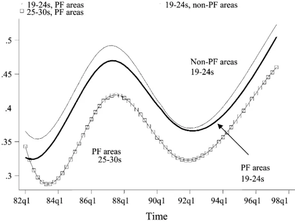
Figure 1 illustrates what is meant by common trends. It refers to the New Deal study described above and compares treated and controls over time with respect to the outflows from unemployment. The common trends assumption holds when the curves for treated and controls are parallel. In our example, the curves are nearly par-allel over most of the period. The only important exception is at the beginning of the observable period. The graph suggests that the common trends assumption on both control groups considered in the study is broadly valid.
The possibility of differential trends motivates the ‘‘differential trend adjusted DID estimator.’’ Suppose we suspect that the common trend assumption of DID does not hold but can assume that selection into treatment is independent of the temporary in-dividual-specific effect,oit, under differential trends
E½uitjdi¼d;t ¼E½nijdi¼d+qdmt
whereqd is a scalar allowing for differential macro effects across the two groups (d
represents the group and is either one or zero).
Figure 1
The DID estimator now identifies
E½aˆDID ¼aATT+ðq1
2q0ÞE½mt12mt0
which does not recover the true ATT unlessq1¼q0, in which case we are back to the
standard DID assumption.
Given the availability of data, one possible solution is to compare the trends of treated and controls historically, prior to the intervention. Historical, prereform data can help if there exists another time interval, sayðt;tÞ (with t,t,k, over which a similar macro trend has occurred. In that case, by comparing the DID esti-mate of the impact of treatment contaminated with the bias from differential trend with the estimate of the differential trend overðt;tÞone can separate the true im-pact of treatment from the differential trend.
More precisely, suppose one finds a prereform period,ðt;tÞfor which the dif-ferential macro trend matches the bias term in the DID estimator,
ðq1
This means that there is a point in history where the relative conditions of the two groups being compared, treatments and controls, evolves similarly to what they do in the prepost reform period, (t0,t1). Together with the absence of policy reforms that
affect the outcome y duringðt;tÞ, this condition allows one to identify the bias termðq1
2q0Þðm
t12mt0Þ by applying DID to that prereform period. The impact of
treatment can now be isolated by comparing DID estimates for the two periods,
ðt0;t1Þ andðt;tÞ. This is the differentially adjusted estimator proposed by Bell, Blundell, and Van Reenen (1999), which will consistently estimate ATT,
ˆ
It is likely that the most recent cycle is the most appropriate, as earlier cycles may have systematically different effects across the target and comparison groups. The similarity of subsequent cycles, and thus the adequacy of differential adjusted DID, can be accessed in the presence of a long history of outcomes for the treatment and control groups.
D. DID with repeated cross-sections: compositional changes
Although DID does not require longitudinal data to identify the true ATT parameter, it does require similar treatment and control groups to be followed over time. In par-ticular, in repeated cross-section surveys the composition of the groups with respect to the fixed effects term must remain unchanged to ensure before-after comparability. If before-after comparability does not hold, the DID will identify a parameter other than ATT. We will illustrate this problem within our running education example.
E. Nonlinear DID models
a dummy variable. In such case, the DID method can conceivably predict probabil-ities outside the ½0,1 range. Instead, the authors suggest using the popular index models and assuming linearity in the index. Unfortunately, DID loses much of its simplicity even under a very simple nonlinear specification.
To extend DID to a nonlinear setting, suppose the outcome equation is now:
yit¼1ðb+aidit+uit.0Þ
ð18Þ
where 1ðAÞ is the indicator function, assuming the value one ifAis true and zero otherwise. As before,
uit¼ni+mt2oit
and the DID assumption holds,
E½uitjdi;t ¼E½nijdi+mt
wheredirepresents the treatment group. Additional assumptions are required. We
as-sume ofollows a distribution F where F is invertible.7 Denote by F21 the inverse
probability rule. We simplify the model further by assuming a common group effect instead of allowing for an individual-specific effect: it is assumed that ni¼nd for
d¼0,1 being the post-program treatment status of individuali8.
Under these conditions and given a particular parametric assumption about the shape of F, say normal, one could think of mimicking the linear DID procedure by just running a probit regression ofyondand dummy variables for group and time (and possibly other exogenous regressorsx) hoping this would identify some average of the treatment parametera. One could then average the impact onyover the treated to recover the average treatment effect on the treated (the individual impact would depend on the point of the distribution where the individual is before treatment).
Unfortunately, this is not a valid approach in general. The problem is that the model contains still another error component which has not been restricted and that, under general conditions, will not fulfill the probit requirements. To see this, notice we can rewrite Model 18 as follows:
yit¼1ðb+aATEdit+ditðai2aATEÞ+nd+mt2oit.0Þ
whereditðai2aATEÞis part of the error term. Standard estimation methods would
re-quire a distributional assumption forðai2aATEÞand its independence from the
treat-ment status.
Instead of imposing further restrictions in the model, we can progress by noticing that under our parametric setup,
E½y0itjdi ¼d;t ¼Fðb+nd+mtÞ
7. More precisely, we are assuming the transitory shocks,o, areiidcontinuous random variables with a strictly increasing cumulative density function, F, which is assumed known.
where, as before,ðy0;y1Þare the potential outcomes in the absence and in the
pres-ence of treatment, respectively. But then the index is recoverable given invertibility of the function F,
b+nd+mt¼F21 E½y0itjdi¼d;t
:
Using this result it is obvious that the trend can be identified from the comparison of nontreated before and after treatment:
mt12mt0¼F21 E½y0itjdi¼0;t12F21 E½y0itjdi¼0;t0:
ð19Þ
Moreover, given the common trend assumption it is also true that, would we be able to observe the counterfactual of interest, E½y0
itjdi¼1;t1
But then Equations 19 and 20 can be combined to form the unobserved counter-factual as follows:
Let the average parameter of interest beaATT, which measures the average impact
among the treated on the inverse transformation of the expected outcomes. Then9 aATT¼F21 E
is generally different from the average index for this group and time period (which isb+aATT+n
1+mt1) given the nonlinearity of F2
1and the
heterog-enous nature of the treatment effect. To see why notice that,
E½y1itjdi¼1;t1 ¼
Z
Dð Þa
Fðb+a+n1+mt1ÞdGajdðajdi¼1Þ
whereDð Þa is the space of possible treatment effects,a, and Gajdis the cumulative distribution function of aamong individuals in treatment groupd. Applying the inverse transformation yields,
F21 E½y1itjdi¼1;t1
E½y0itjdi¼1;t1 ¼F F 21 E½y1itjdi¼1;t12aATT :
Using this expression, the ATT can be estimated by replacing the expected values by their sample analogs,
d
ATT¼y1t12FfF21ð
y1t1Þ2aˆATTg
where
ˆ
aATT¼ ½F21ð y1t1Þ2F21ð
y1t0Þ2½F21ð
yt10Þ2F21ðyt00Þ:
Recently, Athey and Imbens (2006) developed a general nonlinear DID method specially suited for continuous outcomes: the ‘‘changes-in-changes’’ (CIC) estima-tor.10 The discussion of this method is outside the scope of this paper (we refer the interested reader to the original paper by Athey and Imbens 2006).
F. Using DID to estimate returns to education
Since formal education occurs earlier in the lifecycle than labor market outcomes, it is generally not possible to evaluate the returns to education using earnings of treated and controls before and after the treatment. However, in the presence of an exoge-nous change in the environment leading to potential changes in education decisions, one may be able to identify some policy interesting parameter from the comparison of different cohorts. To explore this possibility, we consider the simulation model discussed before but now extended to include an education subsidy.
In this extension to the simple lifecycle model of education investment and work-ing first discussed in Section IIB, the individual lives for three periods correspondwork-ing to basic education, advanced education, and working life. These are denoted by age being zero, one, and two, respectively. The new education subsidy is available to individuals going into advanced education. Eligibility to subsidised education depends on academic performance during basic education as described in more detail below.
At birth, age zero, individuals are heterogeneous with respect to ability, u, and family background,z. At this age all individuals complete basic education and per-form a final test. The score on this test depends on innate ability (u) and the amount of effort (e) the individual decides to put in preparing for it:
si¼g0+g1uiei+qi
ð21Þ
whereqis the unpredictable part of the score andðg0;g1Þare some parameters.
Ef-fortecarries some utility cost, as described in Appendix 1. The (stochastic) payoff to this effort is the possibility of obtaining a subsidy to cover (part of) the cost of ad-vanced education if scoring above a minimum levels.
The remaining of the individual’s life follows as explained before in Section IIB. At age one the individual decides whether to invest in advanced education. In the presence of a subsidy to advanced education the cost is
ci¼d0+d1zi21ðsi.sÞS+vi
ð22Þ
where 1ðAÞis the characteristic function assuming the value one if propositionAis true and zero otherwise.
Finally, age two represents the working life and earnings are realized. The loga-rithm of earnings are defined as in Equation 11:
lnyi¼b0+b1xi+a0di+a1uidi+ui:
1. Specification details and true parameters
For future reference and comparison purposes, we now present a couple of important model parameters along with the true effects. Further specification details can be found in Appendix 1.
The main set of estimates refers to the case where the unobservables in the cost of education (Equation 22) and in the earnings equation (Equation 11) are nega-tively correlated with the correlation coefficient being -0.5. In all cases we will also consider the uncorrelated model, where all selection occurs in the observ-ables. Eligibility to education subsidy is determined by the test score with individ-uals scoring aboves¼4 being eligible. The exogenous explanatory variable,x, is assumed to be discrete, in the present case assuming only two values, zero and one. The exogenous determinant of the cost of education,z, is assumed to follow a truncated normal distribution in the interval ½-2,2. The unobservable level of ability,u, is also assumed to be a truncated normal but this time in the interval
½0,1.
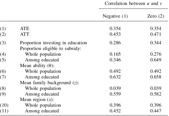
Table 1 presents the true ATE and ATT as well as a range of statistics character-izing the selection process in the presence of an education subsidy. Other parameters and other cases not systematically discussed throughout the paper will be introduced only when relevant. All numbers result from simulations for an economy with an ed-ucation subsidy under the assumption that individuals are perfectly informed about funding opportunities at birth.
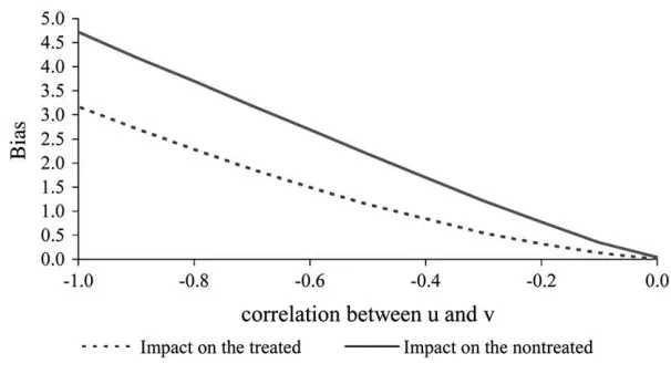
Numbers in Table 1 represent two alternative cases depending on whether the cor-relation between the unobservablesuandvis negative (Column 1) or zero (Column 2). In both cases, the presence of strong selection mechanisms is quite evident. Rows 1 and 2 display the ATE and ATT respectively, and these are markedly different with the average participant benefiting more from advanced education then the average individual. The presence of selection is also suggested by the numbers in Rows 4 to 11 as the average of each variable among the educated is very different from that over the whole population.
2. Sources of variation for DID
This DID application relies on the occurrence of a policy change and availability of individual information collected before and after the policy change. We denote these cohorts by the time of their education decision, namelyt¼0 ort¼1 for whether the education decision is taken before or after the policy change, respectively. We then explore two sources of variability. The first assumes the subsidy is first piloted in one region, sayx¼1, while the old policy remains active in the rest of the country (re-gionx ¼0). The second uses the policy eligibility rule, namely the cutoff point in terms of test score (s), to define treatment and comparison groups. The considered policy change is the introduction of a subsidy for advanced education.
We first discuss the use of pilot studies, with the subsidy being available at time t¼1 in region x¼1 but not in regionx¼0 or at timet ¼0. The question now is: Can we explore this regional change in policy to learn about the returns to edu-cation using DID?
We start by noticing that enrollment into education is not solely determined by the subsidy. Some individuals decide to enroll into education even if no subsidy is avail-able or if not eligible, while some eligible individuals will opt out despite the pres-ence of the subsidy. Thus, there will be some educated individuals even when and
Table 1
Monte Carlo experiment—true effects and selection mechanism
Correlation betweenuandv
Negative (1) Zero (2)
(1) ATE 0.354 0.354
(2) ATT 0.453 0.471
(3) Proportion investing in education 0.286 0.344
Proportion eligible to subsidy:
(4) Whole population 0.165 0.276
(5) Among educated 0.346 0.649
Mean ability (u):
(6) Whole population 0.492 0.492
(7) Among educated 0.632 0.658
Mean family background (z):
(8) Whole population 0.039 0.039
(9) Among educated 0.559 0.582
Mean region (x):
(10) Whole population 0.396 0.396
(11) Among educated 0.452 0.447
where the subsidy is not available. To put it shortly, there is noncompliance. As a result, the ATT will not be identified in general. Instead, what may be identified is the average impact for individuals who change their educational decisions in re-sponse to the subsidy.
To estimate the returns to education among individuals that change education sta-tus in response to the subsidy, we further assume a monotonicity condition—that the chance of assessing subsidized education does not lead anyone to give up education. Instead, it makes education more attractive for all eligibles and does not change the incentives to invest in education among noneligibles.11
Define the treatment and control groups as those living in regions affected (x¼1) and not affected (x¼0) by the policy change and suppose we dispose of information on education attainment and earnings of both groups before and after the policy change. We can then compare the two regions over time using DID.
Designate by lnyxtthe average log earnings in regionxat timet. As before,ditis a
dummy variable indicating whether individualiin cohortthas acquired high educa-tion, and we define the probabilities
pxt¼P dð it¼1jx;tÞ
where againiindexes individuals,xrepresents the region (x¼0,1) andtrepresents time (t¼0,1). Thus,pxtis the odds of participation in regionxat timet. The
mono-tonicity assumption, stating that education is at least as attractive in the presence of the subsidy, implies thatdi1$di0for alliin regionx¼1 and, therefore,p11$p10. In
the control region we assumed01¼d00 for simplicity, ruling out macro trends.12
Assuming the decomposition of the error term as in Assumption DID1,
uit¼ni+mt+oit
yields, under the DID assumptions,
E lny112lny10
¼ ðm12m0Þ+ðp112p10ÞE½aijdi1¼1;di0¼0;xi¼1
The above expression suggests that only the impact on the movers may be identified. Similarly,
E lny012lny00
¼ ðm12m0Þ
since individuals in the control region do not alter their educational decisions. Thus, under the DID assumption we identify,
E½aˆDID ¼ ðp
112p10ÞE½aijdi1¼1;di0¼0;xi¼1:
ð23Þ
Equation 23 shows that the mean return to education on individuals moving into ed-ucation in response to the subsidy can be identified by dividing the DID estimator by the proportion of movers in the treated region,p112p10. This is the LATE parameter.
11. We discuss this type of monotonicity assumption in more detail later on, along with the LATE param-eter.
Not correcting for the proportion of movers implies that a different parameter is estimated: Theaverage impact of introducing an education subsidy on the earnings of the treated, in this case the individuals living in region one. This is a mixture of a zero effect for individuals in the treated region that do not move and the return to education for the movers.13
Under homogeneous treatment effects, all average parameters are equal and thus ATE and ATT are also identified. However, under heterogeneous treatment effects only the impact on the movers can be identified and even this requires especial ditions. In this example we have ruled out movers in the control regions. If other con-ditions differentially affect the educational decisions in nontreated regions before and after the policy intervention, movements are expected among the controls as well. Whether the monotonicity assumption mentioned above holds for the control group or not depends on the circumstances that lead these individuals to move. For simplicity, assume monotonicity holds in control areas such that di1$di0 fori
in the control region. DID will then identify
E½aˆDID ¼ ðp
112p10ÞE½aijdi1¼1;di0¼0;xi¼1
+ðp012p00ÞE½aijdi1¼1;di0¼0;xi¼0:
Now the ability to single out the returns to education on a subset of the movers (movers in regionx¼1 net of movers in regionx¼0) depends on two additional factors: (i) That movers in regionx¼1 in the absence of a policy change would have the same returns to education as movers in region x¼0, which typically requires that they are similar individuals; and (ii) that different proportions of individuals move in the two areas.
Now suppose that instead of a pilot study, we are exploring the use of a global, country-wide policy change. Instead of using treated and nontreated regions, one can think of using the eligibility rules as the source of randomization. The treatment and control groups are now composed of individuals scoring above and below the eligibility thresholds, respectively. Let ˜sdenote eligibility: ˜sis one ifs$sand is zero otherwise. Again, we assume data is available on two cohorts, namely those af-fected and unafaf-fected by the policy change.
The use of the eligibility rule instead of regional variation suffers, in this case, from one additional problem: the identification of the eligibility group before the in-troduction of the program. The affected generations will react to the new rules, adjusting their behavior even before their treatment status is revealed (which amounts to becoming eligible to the subsidy). In our model, future eligibility can be influenced in anticipation by adjusting effort at age zero. As a consequence, a change in the selection mechanism in response to the policy reform will affect the size and composition of the eligibility groups over time. This means that eligibles and noneligibles are not comparable over time and since we are confined to use re-peated cross-sections to evaluate the impact of education, it would exclude DID as a