Full Terms & Conditions of access and use can be found at
http://www.tandfonline.com/action/journalInformation?journalCode=ubes20
Download by: [Universitas Maritim Raja Ali Haji], [UNIVERSITAS MARITIM RAJA ALI HAJI
TANJUNGPINANG, KEPULAUAN RIAU] Date: 11 January 2016, At: 20:48
Journal of Business & Economic Statistics
ISSN: 0735-0015 (Print) 1537-2707 (Online) Journal homepage: http://www.tandfonline.com/loi/ubes20
Feature Screening for Ultrahigh Dimensional
Categorical Data With Applications
Danyang Huang, Runze Li & Hansheng Wang
To cite this article: Danyang Huang, Runze Li & Hansheng Wang (2014) Feature Screening for Ultrahigh Dimensional Categorical Data With Applications, Journal of Business & Economic Statistics, 32:2, 237-244, DOI: 10.1080/07350015.2013.863158
To link to this article: http://dx.doi.org/10.1080/07350015.2013.863158
Accepted author version posted online: 13 Nov 2013.
Submit your article to this journal
Article views: 312
View related articles
Feature Screening for Ultrahigh Dimensional
Categorical Data With Applications
Danyang H
UANGDepartment of Business Statistics and Econometrics, Guanghua School of Management, Peking University, Beijing 100871, P.R. China ([email protected])
Runze L
IDepartment of Statistics and the Methodology Center, The Pennsylvania State University, University Park, PA 16802 ([email protected])
Hansheng W
ANGDepartment of Business Statistics and Econometrics, Guanghua School of Management, Peking University, Beijing 100871, P.R. China ([email protected])
Ultrahigh dimensional data with both categorical responses and categorical covariates are frequently en-countered in the analysis of big data, for which feature screening has become an indispensable statistical tool. We propose a Pearson chi-square based feature screening procedure for categorical response with ultrahigh dimensional categorical covariates. The proposed procedure can be directly applied for detection of important interaction effects. We further show that the proposed procedure possesses screening con-sistency property in the terminology of Fan and Lv (2008). We investigate the finite sample performance of the proposed procedure by Monte Carlo simulation studies and illustrate the proposed method by two empirical datasets.
KEY WORDS: Pearson’s chi-square test; Screening consistency; Search engine marketing; Text classification.
1. INTRODUCTION
Since the seminal work of Fan and Lv (2008), feature screen-ing for ultrahigh dimensional data has received considerable attention in the recent literature. Wang (2009) proposed the forward regression method for feature screening in ultrahigh
dimensional linear models. Fan, Samworth, and Wu (2009) and
Fan and Song (2010) developed sure independence screening
(SIS) procedures for generalized linear models and robust linear
models. Fan, Feng, and Song (2001) developed nonparametric
SIS procedure for additive models. Li et al. (2012) developed a rank correlation based SIS procedure for linear models. Liu,
Li, and Wu (2014) developed an SIS procedure for varying
coefficient model based on conditional Pearson’s correlation. Procedures aforementioned are all model-based methods. In the analysis of ultrahigh dimensional data, it would be very challenging in specifying a correct model in the initial stage.
Thus, Zhu et al. (2011) advocated model-free procedures and
proposed a sure independence and ranking screening
proce-dure based on multi-index models. Li, Zhong, and Zhu (2012)
proposed a model-free SIS procedure based on distance
cor-relation (Szekely, Rizzo, and Bakirov 2007). He, Wang, and
Hong (2013) proposed a quantile-adaptive model-free SIS for
ultrahigh dimensional heterogeneous data. Mai and Zou (2013) proposed an SIS procedure for binary classification with ultra-high dimensional covariates based on Kolmogorov’s statistic. The aforementioned methods implicitly assume that predictor variables are continuous. Ultrahigh dimensional data with cat-egorical predictors and catcat-egorical responses are frequently en-countered in practice. This work aims to develop a new SIS-type procedure for this particular situation.
This work was partially motivated by an empirical analysis of data related to search engine marketing (SEM), which is also referred to as paid search advertising. It has been a standard practice to make textual advertisements on search engines such as Google in USA and Baidu in China. Keyword management plays a critical role in textual advertisements and therefore is of particular importance in SEM practice. Specifically, to max-imize the amount of potential customers, the SEM practitioner typically maintains a large number of relevant keywords. De-pending on the business scale, the total number of keywords ranges from thousands to millions. Practically managing so many keywords is a challenging task. For an easy management, the keywords need to be classified into fine groups. This is a requirement enforced by all major search engines (e.g., Google and Baidu). Ideally, the keywords belong to the same group should bear similar textual formulation and semantic meaning. This is a nontrivial task demanding tremendous efforts and ex-pertise. The current industry practice largely relies on human forces, which is expensive and inaccurate. This is particularly true in China, which has the largest emerging SEM market in the world. Then, how to automatically classify Chinese keywords into prespecified groups becomes a problem of great impor-tance. Such a problem indeed is how to handle high-dimensional categorical feature construction and how to identify important features.
© 2014American Statistical Association Journal of Business & Economic Statistics
April 2014, Vol. 32, No. 2 DOI:10.1080/07350015.2013.863158
237
238 Journal of Business & Economic Statistics, April 2014
From statistical point of view, we can formulate the problem as follows. We treat each keyword as a sample and index it byi with 1≤i≤n. Next, letYi∈ {1,2, . . . , K}be the class
label. We next convert the textual message contained in each keyword to a high-dimensional binary indicator. Specifically, we collect a set of most frequently used Chinese characters
and index them byj with 1≤j ≤p. Define a binary
indica-torXij asXij =1 if the jth Chinese character appears in the
ith keyword andXij =0 otherwise. Collect all those binary
in-dicators by a vectorXi =(Xi1, . . . , Xip)⊤∈Rp. Because the
total number of Chinese characters is huge, the dimension ofXi
(i.e.,p) is ultrahigh. Subsequently, the original problem about keyword management becomes an ultrahigh dimensional classi-fication problem fromXitoYi. Many existing methods,
includ-ingk-nearest neighbors (Hastie, Tibshirani, and Friedman2001,
kNN), random forest (Breiman2001, RF), and support vector
machine (Tong and Koller2001; Kim, Howland, and Park2005,
SVM) can be used for high-dimensional binary classification. However, these methods become unstable if the problem is ul-trahigh dimensional. As a result, feature screening becomes indispensable.
This article aims to develop a feature screening procedure for multiclass classification with ultrahigh dimensional categorical predictors. To this end, we propose using Pearson’s chi-square (PC) test statistic to measure the dependence between categori-cal response and categoricategori-cal predictors. We develop a screening procedure based on the Pearson chi-square test statistic. Since the Pearson chi-square test can be directly calculated using most statistical software packages. Thus, the proposed procedure can be easily implemented in practice. We further study the theoret-ical property of the proposed procedure. We rigorously prove that, with overwhelming probability, the proposed procedure can retain all important features, which implies the sure inde-pendence screening (SIS) property in the terminology of Fan and Lv (2008). In fact, under certain conditions, the proposed method can correctly identify the true model consistently. For convenience, the proposed procedure is referred to as PC-SIS, which possesses the following virtues.
The PC-SIS is a model-free screening procedure because the implementation of PC-SIS does not require one to specify a model for the response and predictors. This is an appealing property since it is challenging to specify a model in the ini-tial stage of analyzing ultrahigh dimensional data. The PC-SIS can be directly applied for multicategorical response and mul-ticategorical predictors. The PC-SIS has excellent capability in detecting important interaction effects by creating new categori-cal predictors for interactions between predictors. Furthermore, the PC-SIS is also applicable for multiple response and grouped or multivariate predictors by defining a new univariate categori-cal variable for the multiple response or the grouped predictors. Finally, by appropriate categorization, PC-SIS can handle the situation with both categorical and continuous predictors. In summary, the PC-SIS provides a unified approach for feature screening in ultrahigh dimensional categorical data analysis. We conduct Monte Carlo simulation to empirically verify our theoretical findings and illustrate the proposed methodology by two empirical datasets.
The rest of this article is organized as follows. Section 2
describes the detailed procedure of PC-SIS and establishes its
theoretical property. Section3presents some numerical studies. Section4presents two real-world applications. The conclusion remark is given in Section5. Technical proofs are given in the Appendix.
2. THE PEARSON CHI-SQUARE TEST BASED SCREENING PROCEDURE
2.1 Sure Independence Screening
Let Yi ∈ {1, . . . , K} be the corresponding class label, and Xi =(Xi1, . . . , Xip)⊤∈Rp be the associated categorical
pre-dictor. Since the predictors involved in our intended SEM ap-plication are binary, we assume thereafter thatXij is binary.
This allows us to slightly simplify our notation and technical proofs. However, the developed method and theory can be read-ily applied to general categorical predictors. Define a generic notationS = {j1, . . . , jd}to be a model withXij1, . . . , Xijd
in-cluded as relevant features. Let|S| =d be the model size. Let
Xi(S)=(Xij :j ∈S)∈R|S| be the subvector ofXi according
toS. DefineD(Yi|Xi(S)) to be the conditional distribution ofYi
givenXi(S). Then a candidate modelSis called sufficient, if
D(Yi|Xi)=DYi|Xi(S). (2.1)
Obviously, the full modelSF = {1,2, . . . , p}is sufficient. Thus, we are only interested in the smallest sufficient model. Theoret-ically, we can consider the intersection of all sufficient models. If the intersection is still sufficient, it must be the smallest. We call it the true model and denote it byST. Throughout the rest
of this article, we assumeST exists with|ST| =d0.
The objective of feature screening is to find a model estimate
Ssuch that: (1)S⊃ST; and (2) the size of|S|is as small as
pos-sible. To this end, we follow the marginal screening idea of Fan and Lv (2008) and propose the Pearson chi-square type statis-tic as follows. DefineP(Yi =k)=πyk,P(Xij =k)=πj k, and
chi-square type statistic can be defined as
which is a natural estimator of
j =
Obviously, those predictors with largerjvalues are more likely
to be relevant. As a result, we can estimate the true model by
S= {j :j > c}, wherec >0 is some prespecified constant.
For convenience, we refer toSas a PC-SIS estimator.
Remark 1. As one can see, Scan be equivalently defined
in terms ofp-value. Specifically, definePj =P(χK2−1> nˆj),
where χK2−1 stands for a chi-squared distribution with K−1 degrees of freedom. BecausePj is a monotonically decreasing
function in j, Scan be equivalently expressed as S= {j :
Pj < pc}for some constant 0< pc<1. For situations in which
the number of categories involved by each predictor is different,
the predictor involving more categories is likely to be associated
with larger j values, regardless of whether the predictor is
important or not. In such cases, directly usingj for variable
screening is less accurate. Instead, it is more appropriate to usep-value Pj obtained from the Pearson chi-squared test of
independence with degrees of freedom (K−1)(Rj −1) for an Rj-level categorical predictor.
2.2 Theoretical Properties
We next investigate the theoretical properties ofS. Define
ωk1k2
j =cov{I(Yi =k1), I(Xij =k2)}. We then assume the
fol-lowing conditions.
(C1) (Response Probability) Assume that there exist two
positive constants 0< πmin< πmax<1 such thatπmin<
πyk< πmax for every 1≤k≤K andπmin< πj k < πmax
for every 1≤j ≤pand 1≤k≤K.
(C2) (Marginal Covariance) Assumej =0 for anyj ∈ST.
We further assume that there exists positive constantωmin,
such that minj∈STmaxk1k2(ω
Condition (C1) excludes those features with one particular cat-egory’s response probability extremely small (i.e.,πyk≈0) or
extremely large (i.e.,πyk≈1). Condition (C2) requires that, for
every relevant categorical featurej ∈ST, there exists at least
one response category (i.e.,k1) and one feature category (i.e.,
k2), which are marginally correlated (i.e.,ωkj1k2> ωmin). Under
a linear regression setup, similar condition was also used by Fan and Lv (2008) but in terms of the marginal covariance. Condi-tion (C2) also assumes thatj =0 for everyj ∈ST. With the
help of this condition, we can rigorously show thatSis selection
consistent forST, that isP(S=ST)→1 asn→ ∞in
The-orem 1. If this condition is removed, the conclusion becomes screening consistent (Fan and Lv2008), that isP(S⊃ST)→1
asn→ ∞. Finally, condition (C3) allows the feature dimension
pto diverge at an exponentially fast speed in terms of the sample sizen. Accordingly, the feature dimension could be much larger than sample sizen. Then, we have the following theorem.
Theorem 1. (Strong Screening Consistency) Under
Condi-tions (C1)–(C3), there exists a positive constant c such that
P(S=ST)→1.
2.3 Interaction Screening
Interaction detection is important for the intended SEM ap-plication. Consider two arbitrary featureXij1 andXij2. We say
they are free of interaction effect if conditioning onYi, they
are independent with each other. Otherwise, we say they have nontrivial interaction effect. Theoretically, such an interaction effect can be conveniently measured by
j1j2=
Subsequently,j1j2can be estimated by
Accordingly, those interaction terms with large j1j2 values
should be considered as promising ones. As a result, it is natural to select important interaction effects byI = {(j1, j2) :j
1j2> c}for some critical valuec >0. It is remarkable that the critical valuecused here is typically different from that ofS. As one
can imagine, searching for important interaction effects over every possible feature pair is computationally expensive. To save computational cost, we suggest to focus on those features inS. This leads to the following practical solution:
I=(j1, j2) :j1j2> candj1, j2∈S. (2.4)
Under appropriate conditions, we can also show that I(I=
IT)→ ∞asn→ ∞, whereIT = {(j1, j2) :j
1j2 >0}.
2.4 Tuning Parameter Selection
We first consider tuning parameter selection for S. To this
end, various nonnegative values can be considered forc. This leads to a set of candidate models, which are collected by a solution pathF = {Sj : 1≤j ≤p}, whereSj = {k1, . . . , kj}.
Here{k1, . . . , kp}is a permutation of{1, . . . , p}such that ˆk1 ≥
ˆ
k2 ≥ · · · ≥ˆkp. As a result, the original problem about tuning
parameter selection for c is converted into a problem about
model selection for F. To solve the problem, we propose the
following maximum ratio criterion. To illustrate the idea, we
temporarily assume that ST ∈F. Recall that the true model
size is|ST| =d0. We then should have ˆkj/ˆkj+1→pcjj+1for
some positive constantcjj+1>0, as long asj +1≤d0. One
the other side, if j > d0, we should have both ˆj and ˆj+1
converges in probability toward 0. If their convergence rates are comparable, we should have ˆkj/ˆkj+1=Op(1). However, if j =d0, we should have ˆj →p cj for some positive constant cj >0 but ˆj+1→p 0. This makes the ratio ˆkj/ˆkj+1 →p ∞.
This suggests thatd0can be estimated by
ˆ
d =argmax0≤j≤p−1ˆkj
ˆ
kj+1,
where ˆ0 is defined to be ˆ0=1 for the sake of
com-pleteness. Accordingly, the final model estimate is given by
S = {j1, j2, . . . , jdˆ} ∈F. Similar idea also can be used to
esti-mate the interaction modelIand get the interaction model size
ˆ
dI. Our numerical experiments suggest that it works fairly well.
3. SIMULATION STUDIES
3.1 Example 1: A Model Without Interaction
We first consider a simple example without any interaction effect. We generateYi ∈ {1,2, . . . , K}withK=4 andP(Yi =
k)=1/K for every 1≤k≤K. Define the true model to be
ST = {1,2, . . . ,10}with|ST| =10. Next, conditional on Yi,
240 Journal of Business & Economic Statistics, April 2014
Table 1. Probability specification for Example 1
j
θkj 1 2 3 4 5 6 7 8 9 10
k=1 0.2 0.8 0.7 0.2 0.2 0.9 0.1 0.1 0.7 0.7
k=2 0.9 0.3 0.3 0.7 0.8 0.4 0.7 0.6 0.4 0.1
k=3 0.7 0.2 0.1 0.6 0.7 0.6 0.8 0.9 0.1 0.8
k=4 0.1 0.9 0.6 0.1 0.3 0.1 0.4 0.3 0.6 0.4
we generate relevant features asP(Xij =1|Yi=k)=θkj for
every 1≤k≤Kandj ∈ST. Their detailed values are given in
Table 1. Then, for any 1≤k≤Kandj ∈ST, we defineθkj =
0.5. For a comprehensive evaluation, various feature dimensions (p=1000,5000) and sample sizes (n=200,500,1000) are considered.
For each random replication, the proposed maximum ra-tio method is used to select both SandI. Subsequently, the
number of correctly identified main effects CME= |SST|
and incorrectly identified main effects IME= |SSc T| with
Sc
T =SF\ST are computed. The interaction effects are
simi-larly summarized. This leads to the number of correctly and incorrectly identified interaction effects, which are denoted by CIE and IIE, respectively. Moreover, the final model size, that is MS= |S| + |I|, is computed. The coverage percentage, defined
by CP=(|SST| + |IIT|)/(|ST| + |IT|), is recorded. Fi-nally, all those summarizing measures are averaged across the
200 simulation iterations and then reported in Table 2. They
correspond to the rows with the screening method flagged by
S+I. For comparison purpose, the full main effect modelSF
(i.e., the model with all the main effect without interaction) and also the selected main effect modelS(i.e., the model with all
the main effect inSwithout interaction) are also included.
The detailed results are given inTable 2. For a given simula-tion model, a fixed feature dimensionp, and a diverging sample sizen, we find that the CME increases toward |ST| =10 and IME decreases toward 0, and there is no overfitting effect. This result corroborates the theoretical result of Theorem 1 very well. In the meanwhile, since there is no interaction in this particular model, CIE is 0 and IIE converges toward 0 asngoes to infinity.
3.2 Example 2: A Model With Interaction
We next investigate an example with genuine interaction ef-fects. Specifically, the class label is generated in the same way
as the previous example withK=4. Conditional onYi=k,
we generateXij withj ∈ {1,3,5,7}according to probability P(Xij =1|Yi =k)=θkj, whose detailed values are given in
Table 3. Conditional onYi andXi,2m−1, we generateXi,2m
ac-cording to
P(Xi,2m =1|Yi =k, Xi,2m−1=0)=0.05I(θk,2m−1≥0.5)
+0.4I(θk,2m−1<0.5)
P(Xi,2m =1|Yi =k, Xi,2m−1=1)=0.95I(θk,2m−1≥0.5)
+0.4I(θk,2m−1<0.5),
Table 2. Example 1 detailed simulation results
Main effect Interaction effect
p n Method CME IME CIE IIE MS CP%
1000 200 SF 10.0 990.0 0.0 0.0 1000.0 100.0
S 9.8 0.0 0.0 0.0 9.9 98.6
S+I 9.8 0.0 0.0 1.1 11.0 98.6
500 SF 10.0 990.0 0.0 0.0 1000.0 100.0
S 10.0 0.0 0.0 0.0 10.0 100.0
S+I 10.0 0.0 0.0 0.2 10.2 100.0
1000 SF 10.0 990.0 0.0 0.0 1000.0 100.0
S 10.0 0.0 0.0 0.0 10.0 100.0
S+I 10.0 0.0 0.0 0.0 10.0 100.0
5000 200 SF 10.0 4990.0 0.0 0.0 5000.0 100.0
S 9.6 0.0 0.0 0.0 9.6 96.6
S+I 9.6 0.0 0.0 1.1 10.7 96.6
500 SF 10.0 4990.0 0.0 0.0 5000.0 100.0
S 10.0 0.0 0.0 0.0 10.0 100.0
S+I 10.0 0.0 0.0 0.8 10.8 100.0
1000 SF 10.0 4990.0 0.0 0.0 5000.0 100.0
S 10.0 0.0 0.0 0.0 10.0 100.0
S+I 10.0 0.0 0.0 0.0 10.0 100.0
Table 3. Probability specification for Example 2
j
θkj 1 3 5 7
k=1 0.8 0.8 0.7 0.9
k=2 0.1 0.3 0.2 0.3
k=3 0.7 0.9 0.1 0.1
k=4 0.2 0.1 0.9 0.7
for every 1≤k≤K and m∈ {1,2,3,4}. Finally, we define
θkj =0.4 for any 1≤k≤Kandj >8. Accordingly, we should
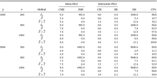
haveST = {1,2, . . . ,8}andIT = {(1,2),(3,4),(5,6),(7,8)}. The detailed results are given inTable 4. The basic findings are qualitatively similar to those inTable 2. The only difference is that the CIE value no longer converges toward 0. Instead,
it converges toward |IT| =4 as n→ ∞ and p fixed. Also,
CP values forSare no longer near 100% since Sonly takes
main effect into consideration. Instead, the CP value forS+Iˆ
converges toward 100% asnincreases andpis fixed.
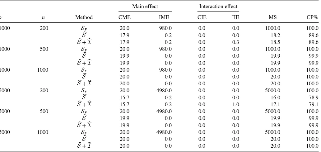
3.3 Example 3: A Model With Both Categorical and Continuous Variables
We consider here an example with both categorical and con-tinuous variables. Fix|ST| =20. Here,Yi ∈ {1,2}is generated
according toP(Yi =1)=P(Yi =2)=1/2. GivenYi =k, we
generate latent variable Zi =(Zi1, Zi2, . . . , Zip)⊤∈Rp with Zij independently distributed asN(μkj,1), whereμkj =0 for
anyj > d0,μkj= −0.5 ifYi=1 andj ≤d0, andμkj =0.5 if Yi =2 andj ≤d0. Finally, we construct observed featureXijas
follows. Ifjis an odd number, we then defineXij =Zij.
Other-wise, defineXij =I(Zij >0). As a result, this example involves
a total ofd0=20 features are relevant. Half of them are
contin-uous and half of them are categorical. To apply our method, we need to first discretize the continuous variables to be categori-cal. Specifically, letzαstands for theαth quantile of a standard
normal distribution. We then redefine those continuous predic-tors as Xij =1 if Xij < z0.25, Xij =2 if z0.25 < Xij < z0.50,
Xij =3 ifz0.50< Xij < z0.75, andXij =4 ifXij > z0.75. By
doing so all the features become categorical. We next apply our method to the converted datasets by usingp-values as described in the Remark 1. The experiment is replicated in a similar man-ner as before with detailed results summarized inTable 5. The results are qualitatively similar to those in Example 1.
4. REAL DATA ANALYSIS
4.1 A Chinese Keyword Dataset
The data contain a total of 639 keywords (i.e., samples), which are classified intoK =13 categories. The total number of
Chi-nese characters involved is p=341. For each class, we
ran-domly split the sample into two parts with equal sizes. One part is used for training and the other for testing. The sample size of the training data isn=320. Based on the training data, models are selected by the proposed PC-SIS method and various clas-sification methods (i.e.,kNN, SVM, and RF) are applied. Their forecasting accuracies are examined on the testing data. For a reliable evaluation, such an experiment is randomly replicated 200 times. The detailed results are given inTable 6. As seen,
the PC-SIS estimated main effect modelS, with size 14.6 on
average, consistently outperforms the full modelSF, regardless
of the classification method. The relative improvement margin
could be as high as 87.2%−51.1%=36.1% for SVM. Such
an outstanding performance can be further improved by includ-ing about 22.3 interaction effects. The maximum improvement margin is 78.0%−67.6%=10.4% for RF.
Table 4. Example 2 detailed simulation results
Main effect Interaction effect
p n Method CME IME CIE IIE MS CP%
1000 200 SF 8.0 992.0 0.0 0.0 1000.0 66.6
S 5.4 0.0 0.0 0.0 5.4 45.7
S+I 5.4 0.0 1.4 5.0 12.0 58.2
500 SF 8.0 992.0 0.0 0.0 1000.0 66.6
S 7.8 0.0 0.0 0.0 7.8 65.5
S+I 7.8 0.0 3.8 1.1 12.8 97.8
1000 SF 8.0 992.0 0.0 0.0 1000.0 66.6
S 8.0 0.0 0.0 0.0 8.0 66.6
S+I 8.0 0.0 4.0 0.2 12.2 100.0
5000 200 SF 8.0 4992.0 0.0 0.0 5000.0 66.6
S 4.9 0.0 0.0 0.0 4.9 41.2
S+I 4.9 0.0 0.9 4.0 9.9 49.5
500 SF 8.0 4992.0 0.0 0.0 5000.0 66.6
S 7.5 0.0 0.0 0.0 7.5 63.1
S+I 7.5 0.0 3.5 1.7 12.8 92.9
1000 SF 8.0 4992.0 0.0 0.0 5000.0 66.6
S 7.9 0.0 0.0 0.0 7.9 66.6
S+I 7.9 0.0 3.9 0.2 12.2 99.9
242 Journal of Business & Economic Statistics, April 2014
Table 5. Example 3 detailed simulation results
Main effect Interaction effect
p n Method CME IME CIE IIE MS CP%
1000 200 SF 20.0 980.0 0.0 0.0 1000.0 100.0
S 17.9 0.2 0.0 0.0 18.2 89.6
S+I 17.9 0.2 0.0 0.3 18.5 89.6
1000 500 SF 20.0 980.0 0.0 0.0 1000.0 100.0
S 19.9 0.0 0.0 0.0 19.9 99.9
S+I 19.9 0.0 0.0 0.0 19.9 99.9
1000 1000 SF 20.0 980.0 0.0 0.0 1000.0 100.0
S 20.0 0.0 0.0 0.0 20.0 100.0
S+I 20.0 0.0 0.0 0.0 20.0 100.0
5000 200 SF 20.0 4980.0 0.0 0.0 5000.0 100.0
S 15.7 0.2 0.0 0.0 16.0 78.9
S+I 15.7 0.2 0.0 1.0 17.1 79.1
5000 500 SF 20.0 4980.0 0.0 0.0 5000.0 100.0
S 19.9 0.0 0.0 0.0 19.9 99.9
S+I 19.9 0.0 0.0 0.0 19.9 99.9
5000 1000 SF 20.0 4980.0 0.0 0.0 5000.0 100.0
S 20.0 0.0 0.0 0.0 20.0 100.0
S+I 20.0 0.0 0.0 0.0 20.0 100.0
4.2 Labor Supply Dataset
We next consider a dataset about labor supply. This is an im-portant dataset generously donated by Mroz (1987) and was dis-cussed by Wooldridge (2002). It contains a total of 753 married white women aged between 30 and 60 in 1975. For illustration purpose, we take a binary variableYi ∈ {0,1}as the response
of interest, which indicates whether the woman participated to the labor market or not. The dataset contains a total of 77 predictive variables with interaction terms included. These vari-ables were observed for both participated and nonparticipated
women. They are recorded by Xi. Understanding the
regres-sion relationship betweenXiandYiis useful for calculating the
propensity score for a woman’s employment decision (Rosen-baum and Rubin1983). However, due to its high dimensionality, directly using all the predictors for propensity score estimation is suboptimal. Thus, we are motivated to apply our method for variable screening.
Following similar strategy, we randomly split the dataset into two parts with equal sizes. One part is used for training and the other for testing. We then apply PC-SIS method to the train-ing dataset. Because this dataset involves both continuous and categorical predictors, the method of discretization (as given in
simulation Example 3) is used. We then apply PC-SIS to the discretized dataset, which leads to estimated modelS. Because
the interaction terms with good economical meanings are
al-ready included inXi (Mroz1987), we did not further pursue
the interaction modelI. An usual logistic regression model is
then estimated based on the training dataset, and the resulting model’s forecasting accuracy is evaluated on the testing data in terms of AUC, which is area under the ROC curve (Wang
2007). The definition is given as follows. Let ˆβ be the max-imum likelihood estimator, which is obtained by conducting
a logistic regression model for Yi and Xi but based on the
training data. Denote the testing dataset, which can be further
decomposed as T =T0T1 with T0= {i∈T :Yi =0} and
T1= {i∈T :Yi =1}. Simply speaking,T0 andT1 collect
in-dices of those testing samples with response being 0 and 1, respectively. Then, AUC in Wang (2007) is defined as
AUC= 1
n0n1
{i1∈T1}
{i2∈T0}
I(X⊤i1β > Xˆ ⊤i2βˆ), (4.1)
wheren0andn1are the sample sizes ofT0andT1, respectively.
For comparison purpose, the full modelSFis also evaluated.
For a reliable evaluation, the experiment is randomly replicated
Table 6. Detailed results for search engine marketing dataset
Model Main Interaction Forecasting accuracy %
Method Size Effect Effect kNN SVM RF
SF 341.00 341.00 0.00 76.89 51.13 60.57
S 14.60 14.60 0.00 85.20 87.19 67.55
S+I 36.85 14.60 22.25 86.96 88.66 78.01
200 times. We find that a total of 10.20 features are selected on
average with AUC=98.03%, which is extremely comparable
to that of the full model (i.e., AUC=98.00%) but with substan-tially reduced features. Lastly, we apply our method to the whole dataset, with 10 important main effects identified and no interac-tion is included. The 10 selected main effects are, respectively, family income, after tax full income, wife’s weeks worked last year, wife’s usual hours of work per week last year, actual wife experience, salary, hourly wage, overtime wage, hourly wage from the previous year, and a variable indicating whose hourly wage from the previous year is not 0.
Remark 2. One can also evaluate AUC according to (4.1) but based on the whole sample and then optimize it with respect to an arbitrary regression coefficientβ. This leads to the Maximum Rank Correlation (MRC) estimator, which has been well studied by Han (1987), Sherman (1993), and Baker (2003).
5. CONCLUDING REMARKS
To conclude this article, we discuss here two interesting top-ics for future study. First, as we discussed before, the proposed method and theory can be readily extended to the situation with general categorical predictors. Second, we assume here the num-ber of response classes (i.e.,K) is finite. How to conduct variable selection and screening with a divergingKis theoretically chal-lenging.
APPENDIX: PROOF OF THEOREM 1
The proof of Theorem 1 consists of five steps. First, we show that there exists a lower bound onjfor everyj ∈ST. Second,
we establishjas a uniformly consistent estimator ofjwhich
is over 1≤j ≤p. Last, we argue that there exists a positive constantcsuch thatS=ST with probability tending to 1.
Step 1. By definition, we have ωk1k2
ωmin. These results together make j lower bounded by
ωminπmax−2. We can then definemin =0.5ωminπmax−2 , which is
a positive constant resulting in minj∈STj > min.
Step 2. The proof of uniform consistency for ˆπj kand ˆπyj,k1k2
is similar. As a result, we omit the details of ˆπyj,k1k2. Also,
based on the uniform consistency of ˆπj k and ˆπyj,k1k2, the
uni-form consistency of j needs only some standard argument
using Taylor’s expansion. The technical details ofj’s uniform
consistency are also omitted. We focus on ˆπj konly.
To this end, we defineZi,j k=I(Xij =k)−πj k. By that we
know EZij,k=0, EZ2ij,k=πj k−πj k2 , and |Zij,k| ≤M with M=1. Also, for a fixed pair of (j, k), we know thatZij,k are
independent fori. All those conditions remind us of Bernstein’s inequality, by which we have
P
whereε >0 is an arbitrary positive constant. SinceM=1 and
πj k−πj k2 ≤1/4, the right-hand side of the inequality can
fur-where the first inequality is due to Bonferonni’s inequality. By Condition (C3), the right-hand side of the final inequality goes
to 0 as n→ ∞. Then we have, under Conditions (C1)–(C3),
Their research was supported in part by National Natural Sci-ence Foundation of China (NSFC, 11131002, 11271032), Fox Ying Tong Education Foundation, the Business Intelligence Re-search Center at Peking University, and the Center for Statis-tical Science at Peking University. Wang’s research was also supported in part by the Methodology Center at Pennsylvania State University. His research was supported by National Insti-tute on Drug Abuse (NIDA) grant P50-DA10075. The content is solely the responsibility of the authors and does not necessarily represent the official views of the NIH or NIDA.
[Received April 2013. Revised September 2013.]
REFERENCES
Baker, S. G. (2003), “The Central Role of Receiver Operating Characteris-tics (ROC) Curves in Evaluating Tests for the Early Detection of Cancer,” Journal of the National Cancer Institute, 95, 511–515. [243]
Breiman, L. (2001), “Random Forest,”Machine Learning, 45, 5–32. [238]
244 Journal of Business & Economic Statistics, April 2014
Fan, J., Feng, Y., and Song, R. (2011), “Nonparametric Independence Screen-ing in Sparse Ultra-High Dimensional Additive Models,”Journal of the American Statistical Association, 116, 544–557. [237]
Fan, J., and Lv, J. (2008), “Sure Independence Screening for Ultra-High Di-mensional Feature Space” (with discussion),Journal of the Royal Statistical Society,Series B, 70, 849–911. [237,238,239]
Fan, J., Samworth, R., and Wu, Y. (2009), “Ultrahigh Dimensional Feature Se-lection: Beyond the Linear Model,”Journal of Machine Learning Research, 10, 1829–1853. [237]
Fan, J., and Song, R. (2010), “Sure Independent Screening in Generalized Linear Models With NP-Dimensionality,”The Annals of Statistics, 38, 3567–3604. [237]
Han, A. K. (1987), “Nonparametric Analysis of a Generalized Regression Model,”Journal of Econometrics, 35, 303–316. [243]
Hastie, T., Tibshirani, R., and Friedman, J. (2001),The Elements of Statistical Learning, New York: Springer. [238]
He, X., Wang, L., and Hong, H. G. (2013), “Quantile-Adaptive Model-Free Variable Screening for High-Dimensional Heterogeneous Data,”The Annals of Statistics, 41, 342–369. [237]
Kim, H., Howland, P., and Park, H. (2005), “Dimension Reduction in Text Classification With Support Vector Machines,”Journal of Machine Learning Research, 6, 37–53. [238]
Li, G. R., Peng, H., Zhang, J., and Zhu, L. X. (2012), “Robust Rank Correlation Based Screening,”The Annals of Statistics, 40, 1846–1877. [237] Li, R., Zhong, W., and Zhu, L. (2012), “Feature Screening Via Distance
Cor-relation Learning,”Journal of American Statistical Association, 107, 1129– 1139. [237]
Liu, J., Li, R., and Wu, R. (2014), “Feature Selection for Varying Coefficient Models With Ultrahigh Dimensional Covariates,”Journal of American Sta-tistical Association, 109, DOI: 10.1080/01621459.2013.850086. [237]
Mai, Q., and Zou, H. (2013), “The Kolmogorov Filter for Variable Screen-ing in High-Dimensional Binary Classification,”Biometrika, 100, 229– 234. [237]
Mroz, T. (1987), “The Sensitivity of an Empirical Model of Married Women’s Hours of Work to Economic and Statistical Assumptions,”Econometrica, 55, 765–799. [242]
Rosenbaum, P., and Rubin, D. (1983), “The Central Role of the Propensity Score in Observational Studies for Causal Effects,”Biometrika, 70, 41– 55. [242]
Sherman, R. P. (1993), “The Limiting Distribution of the Maximum Rank Cor-relation Estimator,”Econometrica, 61, 123–137. [243]
Sz´ekely, G. J., Rizzo, M. L., and Bakirov, N. K. (2007), “Measuring and Testing Dependence by Correlation of Distances,”The Annals of Statistics, 35, 2769–2794. [237]
Tong, S., and Koller, D. (2001), “Support Vector Machine Active Learning With Application to Text Classification,”Journal of Machine Learning Research, 2, 45–66. [238]
Wang, H. (2007), “A Note on Iterative Marginal Optimization: A Simple Algo-rithm for Maximum Rank Correlation Estimation,”Computational Statistics & Data Analysis, 51, 2803–2812. [242]
——— (2009), “Forward Regression for Ultra-High Dimensional Variable Screening,”Journal of the American Statistical Association, 104, 1512– 1524. [237]
Wooldridge, J. M. (2002),Econometric Analysis of Cross Section and Panel Data, Cambridge, MA: MIT Press. [242]
Zhu, L. P., Li, L., Li, R., and Zhu, L. X. (2011), “Model-Free Feature Screen-ing for Ultrahigh Dimensional Data,”Journal of the American Statistical Association, 106, 1464–1475. [237]