Pricing Decision Model for Short Life-cycle Product in a
Closed-loop Supply Chain with Remanufacturing
Shu San Gana, c, I Nyoman Pujawana1, Suparnoa, Basuki Widodob
a
Department of Industrial Engineering – Faculty of Industrial Technology,
Sepuluh Nopember Institute of Technology, Surabaya 60111, Indonesia
b
Department of Mathematics – Faculty of Mathematics and Natural Science
Sepuluh Nopember Institute of Technology, Surabaya 60111, Indonesia
c
Department of Mechanical Engineering – Faculty of Industrial Technology,
Petra Christian University, Surabaya 60236, Indonesia
Abstract
While there has been very few published works that attempt to model
remanufacturing decisions for products with short life-cycle, we believe that there are many
situations where remanufacturing short life-cycle products is rewarding economically as well
as environmentally. We propose a model for determining prices that maximize the supply
chain’s total profit.
The system consists of a retailer, a manufacturer, and a collector of used-product
under multi-period setting. Demand functions are time-dependent functions, both for new and
remanufactured products; and price-sensitive. Return rate is an increasing function of the
collecting price. We take pricing game approach, where manufacturer is the leader. The
model is solved analytically to find optimal prices as well as analytical insights.
The results suggest that the optimal price of remanufactured product is higher during
the decline phase compared to the price in previous phases. Numerical examples show that
higher remanufacturing cost-savings has reduced collector’s profit.
Identification: “Sustainable Supply Chain” and “Pricing and Revenue Management”
Keywords: short life cycle product, remanufacturing, closed loop supply chain, pricing,
optimization.
JEL classification: D4 (Market structure and pricing) and C3 (Multiple or Simultaneous
Equation Models; Multiple Variables)
Introduction
Remanufacturing is a process of transforming used product into “like-new” condition,
so there is a process of recapturing the value added to the material during manufacturing
stage (Atasu, Guide, & Wassenhove, 2010; Atasu, Sarvary, & Wassenhove, 2008). The idea
of remanufacturing used products has gained much attention recently for both economical
and environmental reasons. As suggested by Gray & Charter (2008), remanufacturing can
reduce production cost, the use of energy and materials. There are numerous studies on
remanufacturing. However, most of the published works on remanufacturing have considered
durable or semi-durable products. Very little attempt has been made to study how
remanufacturing maybe applied to products with short life-cycle. In some developing
countries like Indonesia, there is a large segment of society that could become potential
market for remanufactured short life-cycle products like mobile phones, computers and
digital cameras.
Several studies show that life-cycle for such high-technology products is getting
shorter due to rapid innovation in technology (Guide, Jayaraman & Linton, 2003; Lebreton &
Tuma, 2006; Wu, Aytac, Berger & Armbruster, 2006; Xianhao & Qizhi, 2007; Briano,
Caballini, Giribone & Revetria, 2010; Hsueh, 2011), but there are limited number of
remanufacturers for these products. In Europe and the United States, the decisions to
remanufacture electronic products are encouraged by government regulations such as WEEE
(2003) and RoHs (2003), and as a form of responsibility for environmental conservation
can provide economic benefits (Lee, Cho & Hong, 2010; Kaebernick, Manmek & Anityasari,
2006; and Kerr & Ryan, 2001). Considering the mounting wastes from electronic products
nowadays, the potential of remanufacturing practices in reducing waste sent to the landfill, as
well as in reducing production costs, we believe it is very important to study issues in
remanufacturing of short life-cycle product in a closed-loop supply chain.
Pricing decision is an important task in an effort to gain economic benefit from
remanufacturing practices. There are several studies focused on pricing of remanufactured
products, but many of them have not considered the whole supply chain, and also only a very
few concern about obsolescence of short life-cycle products. Our study will be focused on
pricing decisions in a closed-loop supply chain involving manufacturer, retailer and collector
of used-products, where customers have the option to purchase new or remanufactured
products in the same market channel. We consider an oligopoly for single item with no
constraint on the quantity of remanufacturable cores throughout the selling horizon.
Literature Review
Remanufacturing of mobile phones and electronic products has been recognized as an
important practice. Helo (2004) claimed that product life-cycle has significantly shortened by
rapid technological advancement, and coupled with fashionable design that attracts frequent
purchases of new products, has generated pressure on and opportunities for reverse logistics.
Franke, Basdere, Ciupek & Seliger (2006) suggested that remanufacturing of durable
extended to a large number of consumer goods with short life-cycle and relatively low values,
like mobile phones and computers. He also quoted market studies by Kharif (2002),
Marcussen (Marcussen, 2003) and Directive 2002/96/EC which revealed that there is a
significant potential for mobile phone remanufacturing due to the large supply market of the
used mobile phones in Europe and the high market demand in Asia and Latin America.
Neto & Bloemhof-Ruwaard (2012) found that remanufacturing significantly reduces
the amount of energy used in the product life-cycle, even though the effectiveness of
remanufacturing is very sensitive to the life span of the second life of the product. They also
proposed that the period of the life-cycle in which the product is returned to recovery, the
quality of the product, the easiness to remanufacture and the recovery costs can affect
whether or not remanufacturing is more eco-efficient than manufacturing. Rathore, Kota &
Chakrabarti (2011) studied the case of remanufacturing mobile handsets in India. They found
that used phone market is very important, even though with a lack of government regulation
for e-wastes. It is also observed that there is a negative user-perception of second hand goods
and that the process of remanufacturing has not been able to capture much required attention
from its stakeholders. J. Wang, Zhao & Wang (2011) showed that the mobile phone market in
China is growing rapidly. The above mentioned studies have affirmed our intuitive
proposition that there is a high potential for remanufacturing short life cycle products.
Motives for deploying reverse chain can be for profitability or environmental impact
mitigation, which either driven by regulation and/or morale. In our research, the underlying
motive considered would be focused on profitability, which seems to be the suitable motive
developing countries. Guide & Wassenhove (2009) suggest that key activities in reverse
supply chain can be categorized as (1) front end, which deals with product returns
management; (2) engine, which covers remanufacturing operations issues; and (3) back end,
which handles market development of remanufactured product. They believe that it is
important to keep business focused in research of closed-loop supply chain for relevance to
industry; hence highlight the significance of profitability, product valuation, pricing and
marketing issues. In terms of marketing strategy, Atasu et al. (2010) concluded that
remanufacturing does not always cannibalize the sales of new products. He proposed that
managers, who understand the composition of their markets and use the proper pricing
strategy, should be able to create additional profit. In a similar manner, Souza (2013) points
out that introducing remanufactured product to the market alongside with the new product
has two implications, namely market expansion effect and cannibalization effect; which
makes pricing of the two products is critical. Therefore, pricing decision is an important task
in an effort to gain economic benefit from remanufacturing practices.
There are several studies that discuss pricing strategies involving remanufactured
products, obsolescence, and nonlinear demand function. However, none has considered the
situation that we address in this paper. Table 1 shows the review result and where our
proposed model stands.
TABLE 1. LITERATURES ON PRICING MODELS
Supply Chain
members involved
Differen-tiating New & Reman
Planning Horizon
Demand Function
Decision variables
Objective Consi-dering obsoles-cence
Remark
Guide et al. (2003)
remanu-facturer
only reman product
single period
Dr known price of * reman * core
max profit no consider several quality classes of
Supply Chain members involved Differen-tiating New & Reman Planning Horizon Demand Function Decision variables Objective Consi-dering obsoles-cence Remark Bakal & Akcali (2006) remanu-facturer only reman product single period
linear in price price of * reman * core
max profit no consider effect of recovery yield Ferrer & Swaminathan (2006) manufac-turer no (Pn = Pr)
* infinite * two period * multi period
linear in price * price * quantity
max profit no consider monopoly & duopoly
Vadde et al. (2006) product recovery facility only reman product selling horizon function of price and obsolescence
* price max profit yes consider 2 types of obsolescence
* gradual * sudden Mitra (2007) retailer reman &
refurbish products
selling horizon
two cases: * linear in
price * non-linear
price of * reman * refurbish
max revenue no consider the availability of
product
Atasu et al. (2008)
manufac-turer
yes (Pn ≠ Pr)
two period linear in price * price * quantity
max profit no consider green segment, market
diffusion, competition with
other OEM Qiaolun et al.
(2008) * manufac-turer * retailer * collector no (Pn = Pr)
selling horizon
linear in price price of * retail *wholesale * collecting
max profit no manufacturer is the Stackelberg leader
Li et al. (2009) remanufac-turer only reman product single period stochastic, function of price price of * reman *core max utilization
no consider random
yield and random demand Liang et al.
(2009) remanufac-turer only reman product single period
none price of core high return on investment
no consider selling price follows GMB,
and core price follows option principles Ferrer & Swaminathan (2010) manufac-turer yes (Pn ≠ Pr)
* infinite * two period * multi period
linear in price * price * quantity
max profit no consider monopoly & duopoly Ovchinnikov (2011) manufac-turer yes (Pn ≠ Pr)
Pn fixed
selling horizon
Dn known & constant Dr function of
price
* price * quantity
of reman
max profit no also study customers’ switching behavior
α(Pr)∈[0,1] Shi et al.
(2011)
manufac-turer
no (Pn = Pr)
single period
stochastic, linear in price
* price * quantity of
new & reman
max profit no consider understocking & overstocking risks
Vadde et al. (2011) product recovery facility no new products single period
deterministic prices max revenue min cost
no consider several types of used
Supply Chain members involved Differen-tiating New & Reman Planning Horizon Demand Function Decision variables Objective Consi-dering obsoles-cence Remark
Wei & Zhao (2011)
* manufac-turer * retailer
no (Pn = Pr)
single period
linear in price price of * retail *wholesale * collecting
max profit no consider two competing retailers
Pokharel & Liang (2012)
consolidati on center
only cores single period
Dr is known * core price * quantity of cores
min cost no consider stochastic return quantity and
quality Wu (2012a) * OEM
* remanu-facturer
yes (Pn ≠ Pr)
two period linear in price prices * new * reman
max profit no consider level of interchangeability
Wu (2012b) * OEM *
remanu-facturer
yes (Pn ≠ Pr)
* two period * multi period
linear in price prices * new * reman
max profit no consider degree of disassemblability
Chen & Chang (2013)
manufac-turer
yes (Pn ≠ Pr)
* static * 2-period * multi periods over life-cycle *linear in price, with substitutable coefficient *dynamic (over time) price of * new * reman for each period
max profit no *static
unconstrained *dynamic pricing -
constrained * consider system
of manufacturing only & hybrid
settings Jena & Sarmah (2013) *remanu-facturer *retailer only reman product single period
random cores price max profit no consider 3 schemes of collection: direct,
indirect, coordinated Xiong et al.
(2013) manufac-turer only reman product finite & infinite horizon
random cores price min cost no consider lost sales and uncertain quality of used
products proposed model *manufac-turer * retailer * collector yes (Pn ≠ Pr)
selling horizon
function of time and price
price of * retail *wholesale * collecting
max profit yes
Note:
Pn = price of new product, Pr = price of remanufactured product Dn = demand of new product, Dr = demand of remanufactured product
Problem Description
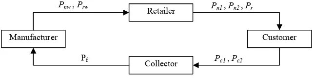
We consider a closed-loop supply chain with three members, manufacturers, retailer,
and collector as depicted in Figure 1. Manufacturer acts as the leader and releases initial
Finally, manufacturer updates the prices to find the optimum ones. The other members then
follow that policy and maintain a balanced quantity along the supply chain.
FIGURE 1. FRAMEWORK OF THE CLOSED-LOOP PRICING MODEL
The product considered in this model is single item, short life-cycle, with
obsolescence effect after a certain period. Demand functions are time-dependent functions
which represent the short life-cycle pattern along the entire phases of product life-cycle, both
for new and remanufactured products; and linear in price. The market demand capacity is
adopted from Wang & Tung (2011), that was constructed based on Verhulst’s population
model and extended to cover the obsolescence period, where the demand decreases
significantly.
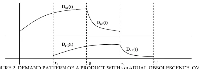
Let the selling horizon be [0, T]. Demand of the remanufactured product starts to
appear at t1∈[0, µ], when some of the products have reached their end-of-use. The cores used
for remanufacturing during [t1, t3] are collected from the returns of new products sold during
[0, µ]. During [t3, T], there are only remanufactured products offered, and the cores come
from new products sold during [µ, t3]. Figure 2 represents the demand pattern over time. The
demand functions for new and remanufactured products can be formulated as follows:
(
)
(
)
λ µλ
δ µ
δ µ λ
µ
U n
Ut n
n
ke D U k where t
t t
U U t D
t ke
U t D t
D −
−
+ =
− =
≤ ≤ +
− =
≤ ≤ +
= =
1
1 / ;
) ( / ) (
0 ; 1
/ ) ( )
( 0
3 2
1
Retailer
Customer Manufacturer
Collector
Pn1, Pn2, Pr
Pc1, Pc2
Pf
(
)
(
)
( )0
3 3
2
3 1
) ( 1
1 3 1
1
1 /
; )
( / ) (
; 1
/ ) ( )
( r V t t
r
t t V r
r
he D V h where T
t t t
t V V t D
t t t he
V t D t
D − −
− −
+ =
− =
≤ ≤ +
− =
≤ ≤ +
=
= η η
ε ε
η
where U is a parameter representing the maximum possible demand, µ is the time when the
demand reaches its peak U level, D0 is the demand when t=0, and λ is the speed of change in
the demand as a function of time. A parallel definition is applicable for V, t3, Dr0, and η
respectively for the remanufactured products.
FIGURE 2. DEMAND PATTERN OF A PRODUCT WITH GRADUAL OBSOLESCENCE, OVER TIME
The new product is sold at retail price Pn1 during [0, µ], and Pn2 during [µ, t3]. Pm is
the maximum price, known and fixed, poses as the upper limit, at which demand would be
zero. Remanufactured product are sold at retail price Pr during [t1, T], and the maximum price
is Pn2, since customer would choose to buy new product rather than remanufactured one
when the remanufactured product price is as high as Pn2. Therefore, demand of new product
during [0, µ] is Dn1(t)(1 – Pn1/Pm), demand of new product during [µ, t3] is Dn2(t)(1 – Pn2/Pm);
demand of remanufactured product during [t1, t3] is Dr1(t)(1 – Pr/Pn2), and demand of
remanufactured product during [t3, T] is Dr2(t)(1 – Pr /Pn2).
The demand function information is shared to all members of the supply chain, and
retailer decides the retail prices (Pn1, Pn2, Pr), manufacturer decides the wholesale prices for new product (Pnw) and remanufactured product (Prw), while collector determines collecting
Dn1(t)
Dn2(t)
Dr 1(t)
Dr 2(t)
price Pc1 and Pc2 for cores collected from new products sold during [0, µ] and [µ, t3]
respectively. Since the product has short life-cycle, remanufacturing process is only applied
to cores originated from new products. Return rate (τ) is an increasing function of the
collecting price. We use the function proposed by Qiaolun et al. (2008), τ1= γ1Pc1θ1 and τ2=
γ2Pc2θ2, where γ1, γ2, θ1, θ2 ∈[0,1]. It is assumed that collector only accepts cores with a
certain quality grade, and all collected cores will be remanufactured. Unit raw material cost
for new product (crw), unit manufacturing cost (cm), unit remanufacturing cost (cr), and unit collecting cost (c) are known and constant, while transfer price Pf is a given value in the model. The objective of the proposed model is to find the optimum prices that maximize total
profit of the supply chain using pricing game approach.
Optimization
After manufacturer releases initial wholesale prices (Pnw, Prw), retailer optimizes the retail prices Pn1, Pn2, and Pr. The profit function can be formulated as follows:
(
)
(
)
(
)
(
P P)
dtP P t t V V dt P P P P he V dt P P P P t U U dt P P P P ke U rw r T t n r rw r t t n r t t V nw n t m n nw n m n Ut R − − + − + − − + + − − + − + − − + = Π
∫
∫
∫
∫
− − − 3 3 1 1 3 2 3 2 ) ( 2 2 1 0 1 1 ) ( 1 1 1 ) ( 1 1 ε µ δ µ λ η µ µ λ(
)
(
) (
)
(
r rw)
n r nw n m n nw n m n P P P P d d P P P P d P P P P
d −
− + + − − + − − = 2 4 3 2 2 2 1 1
1 1 1 1 ... (1)
where
(
)
The objective is to maximize profit (1), and consequently it needs to satisfy the first
derivative condition. Hence,
(
)
/2*
1 m nw
n P P
P = + ……… (2) ; Pr*=
(
Pn2+Prw)
/2 ………….…….… (3)(
)
(
) (
)( )
04 *
4 1
*
2 2 3 4 2
2 4 3 2 3 2 2 = + − + + + + − rw n m nw n m P d d P d d P P d P d
P ………..……. (4)
It is expected that Pn2* is lower than Pn1* to increase demand rate at the decline stage,
however the model allows Pn2* to attain higher value than Pn1*, which in turns is not
attractive for customers. Our preliminary investigation showed that Pn2 has a tendency to
attain higher value than Pn1, which is also consistent with Ferrer & Swaminathan’s finding
(Ferrer & Swaminathan, 2006). Therefore, we impose a constraint where Pn2≤Pn1.
In the collector’s optimization model, the objective function is
(
)
(
P P c)
P P d P c P P P P d
P f c
m n c c f m n c
C − −
− + − − − =
Π 2 2
2 2 2 1 1 1 1
1 1 1
Max γ θ1 γ θ2 …………...(5)
However, since we assume balanced quantity throughout the supply chain, collector
should only collect as much as the demand of the remanufactured product, which
consequently determines collecting prices based on the following equations: (1/ 1)
2 3 1 1 1 1 1 1 * * θ γ − − = n r m n c P P d P P d
P .……..…... (6) ;
(1/ 2)
2 4 2 2 2 2 1 1 * * θ γ − − = n r m n c P P d P P d
P ………..…. (7)
This approach is supported by Guide, Teunter, et al. (2003). When collecting prices
are set, the maximization problem has shifted to a matter of determining the transfer price,
cost saving (s) as a parameter for determining transfer price Pf, such that unit cost for remanufacturing is (1–s) of unit cost for manufacturing. This approach is logical because we believe that savings from remanufacturing would be an appropriate incentive for the
manufacturer to remanufacture a product. After transfer price is agreed upon, manufacturer
will determine the wholesale prices for both the new (Pnw) and the manufactured products (Prw) in order to maximize her profit which is expressed in the following function:
(
) (
)
(
rw f r)
n r m rw nw m n m n
M P P c
P P d d c c P P P d P P
d − −
− + + − − − + − = Π 2 4 3 2 2 1
1 1 1 1 ……..(8)
First derivative conditions for optimizing manufacturer’s profit are
(
)
(
)
(
)
02 1 2 1 1 2 2 2 4 3 2 1 2 2 1 1 = ∂ ∂ − − − + + − − − − − − − + − = ∂ Π ∂ nw n r f rw n r n m rw nw m m rw nw m m n m n nw M P P c P P P P P d d c c P P d c c P P d P P d P P d P ...(9)
(
)
(
)
(
)
(
)
02 1 2 1 2 2 2 4 3 2 2 4 3 2 4 3 = ∂ ∂ − − − + + − − − − − + − − + = ∂ Π ∂ rw n r f rw n r n m rw nw m r f rw n n r rw M P P c P P P P P d d c c P P d c P P P d d P P d d P ...(10) where
(
2 3 4)
2 2 2 2 2 2 2 2
6d P d P P d d d
P d P P m nw n n nw n + + − − = ∂ ∂ ...(11)
(
)
(
)
2(
3 4)
2 2 2 2 2 4 3 2 2 4
12d P d P P P P P d d
P P d d P P n m nw m n n rw m rw n + + + + − + = ∂ ∂ ...(12)
By solving equations (9) and (10), the optimum wholesale price Pnw* and Prw* can be found. However, with these optimum wholesale prices, retailer’s profit can decrease
manufacturer considers demand rate to be influenced by the wholesale prices. In this case,
retailer’s margin rate is assumed, namely m1, m2, and m3for products sold at Pn1, Pn2, and Pr respectively. These margins are treated as parameters to the model. The modified profit
function becomes
(
) (
)
(
rw f r)
nw rw m rw nw m nw m nw
M P P c
P m P m d d c c P P P m d P P m
d − −
− + + − − − + − = Π 2 3 4 3 2 2 1 1
2 1 1 1
………..(13)
The first derivatives are
(
)
(
)
(
)
01 1 2 2 3 4 3 2 2 1 1 2 2 1 1 2 = − − + + − + − + − − + − = ∂ Π ∂ r f rw nw rw m nw m nw m rw nw m nw M c P P P m P m d d P P m d P P m d c c P P d m d m P …………..(14)
(
)
1(
)
1 02 3 2 3 4 3 2 = − + − − + + = ∂ Π ∂ nw rw r f rw nw rw M P m P m c P P P m m d d
P ………..(15)
Solving (14) and (15) will result in the optimum wholesale prices Pnw** and Prw**. Manufacturer applies the wholesale prices to the demand rate provided by retailer. This
recalculation might decrease the total profit of supply chain members since increasing retail
price would decrease the demand rate.
Numerical Example
In this numerical example, let assume that new product’s demand capacity parameters
V=500, Dr0=50, η=0.01. Selling horizon is divided into four time periods where t1=1, µ=2,
t3=3, and T=4. The unit raw material cost for new product crw=1500, unit manufacturing cost
cm=1000, unit remanufacturing cost cr=800, and unit collecting cost c=100. Maximum price
is Pm=12000, and remanufacturing cost saving is 20%. Return rate parameters are γ1= γ2
=0.01, and θ1= θ2=0.7. Manufacturer’s assumption for Retailer’s margins are m1 = m2 = m3 =
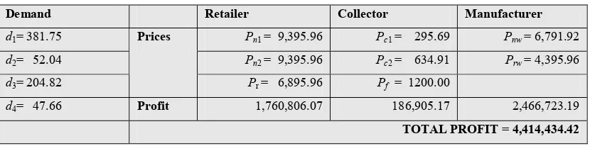
120%. Table 2 shows the numerical example results.
It is observed that Pn2 is higher than Pn1 which forced the system to adjust so that Pn2
does not exceed Pn1. It appears that the rapid decrease in demand for the new product during
[µ, t3] could not be compensated by giving a price discount. Mathematically it is
understandable that when there is a rapid decline in demand and reducing price does not lead
to a significant increase in demand, the only way to maintain profit is to set the retail price
high. However, from business perspective it does not make good sense to increase the retail
price when a product is entering a decline stage. We also observed that collector profit is
much lower than retailer’s and manufacturer’s, because collector only gains from
remanufactured product. This result is consistent with Qiaolun et al. (2008).
TABLE 2. NUMERICAL EXAMPLE RESULTS
Demand Retailer Collector Manufacturer
d1= 381.75 Pn1 = 9,395.96 Pc1 = 295.69 Pnw= 6,791.92
d2= 52.04 Pn2 = 9,395.96 Pc2 = 634.91 Prw = 4,395.96
d3= 204.82
Prices
Pr = 6,895.96 Pf = 1200.00
d4= 47.66 Profit 1,760,806.07 186,905.17 2,466,723.19
TOTAL PROFIT = 4,414,434.42
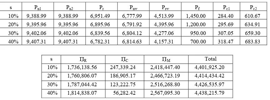
Remanufacturing cost saving obviously has an impact on collector’s and
manufacturer’s profit, and it affects the total profit. By varying s from 10%, 20%, 30% and 40%, we find that the total profit is increasing along with higher s. This relations can be explained as follows. When higher s is used, the remanufacturing variable cost is lower,
hence the margin for each remanufactured product is higher. Hence, the ratailer could set
lower retail price for remanufactured products. As Table 3 shows, with higher s values, the optimum value of Pr decreases which then creates higher demand for remanufactured products. However, collector’s profit diminishes as s increases, so a limit should be posted according to both parties agreement.
TABLE 3. THE EFFECT OF REMANUFACTURING COST SAVINGS ON OPTIMUM RESULTS
s Pn1 Pn2 Pr Pnw Prw Pf Pc1 Pc2
10% 9,388.99 9,388.99 6,951.49 6,777.99 4,513.99 1,450.00 284.40 610.67 20% 9,395.96 9,395.96 6,895.96 6,791.92 4,395.96 1,200.00 295.69 634.91 30% 9,402.06 9,402.06 6,839.56 6,804.12 4,277.06 950.00 307.05 659.30 40% 9,407.31 9,407.31 6,782.31 6,814.63 4,157.31 700.00 318.47 683.83
s ΠR ΠC ΠM Total
10% 1,736,138.56 247,339.24 2,418,447.40 4,401,925.20 20% 1,760,806.07 186,905.17 2,466,723.19 4,414,434.42 30% 1,787,044.42 123,222.75 2,516,268.80 4,426,535.97 40% 1,814,838.07 56,282.42 2,567,095.30 4,438,215.79
Conclusion and Future Research Opportunities
In this study we have developed pricing model for short life-cycle with
remanufacturing. The study fills the gap in remanufacturing literature which to date has been
mostly dominated by durable products. For some short life-cycle products, remanufacturing
should be quick as the demand for the product is diminishing fast. The lack of coordination in
making the pricing decision has led the model to set too high retal prices and hence the
demand potential is not well exploited. We initially thought that the retail price should be
reduced when the product is entering a decline phase, but from the results it is apparent that
lowering the price does not help increasing the profit during that period. This is also
understandable because as the demand is sharply declining, the only way to obtain higher
profit is to set a high price, so getting a very few customers that are buying the product with
high price results in higher revenue rather than discounting the price, but the demand only
increases slightly. However, from business point of view, it is not sensible to increase the
price during the decline period. Numerical examples show that higher remanufacturing
cost-savings has reduced collector’s profit, which means retailer or manufacturer should take over
the collection activities under high remanufacturing cost-savings cases.
Future research may be directed toward development of models that consider different
demand processes, multiple objective functions, and the case when balanced quantity is not
the case. It may be possible that the collector is not able to collect at the quantity desired by
the manufacturer. It is also possible that the manufacturer has a certain capacity constraint
where not all demand can be satisfied. In such as case it is important to take into account the
References
1. Atasu, A., Guide, V. D. R. J., & Wassenhove, L. N. V. (2010). So what if remanufacturing cannibalizes my new product sales? California Management Review, 52(2), 56-76. doi:10.1525/cmr.2010.52.2.56 2. Atasu, A., Sarvary, M., & Wassenhove, L. N. V. (2008). Remanufacturing as a marketing strategy.
Management Science, 54(10), 1731-1746.
3. Bakal, I. S., & Akcali, E. (2006). Effects of Random Yield in Remanufacturing with Price-Sensitive Supply and Demand. Production and Operations Management, 15(3), 407-420.
4. Briano, E., Caballini, C., Giribone, P., & Revetria, R. (2010). Using a System Dynamics Approach for Designing and Simulation of Short Life-Cycle Products Supply Chain. In S. Lagakos, L. Perlovsky, M. Jha, B. Covaci, A. Zaharim, & N. Mastorakis (Eds.), CEA’10 Proceedings of the 4th WSEAS international conference on Computer engineering and applications (pp. 143-149). World Scientific and Engineering Academy and Society (WSEAS) Stevens Point, Wisconsin, USA ©2009.
5. Chen, J.-M., & Chang, C.-I. (2013). Dynamic pricing for new and remanufactured products in a closed-loop supply chain. Intern. Journal of Production Economics. Elsevier. doi:10.1016/j.ijpe.2013.06.017 6. Chung, C.-J., & Wee, H.-M. (2011). Short life-cycle deteriorating product remanufacturing in a green
supply chain inventory control system. International Journal of Production Economics, 129(1), 195-203. Elsevier. doi:10.1016/j.ijpe.2010.09.033
7. Ferrer, G., & Swaminathan, J. M. (2006). Managing New and Remanufactured Products. Management Science, 52(1), 15-26.
8. Ferrer, G., & Swaminathan, J. M. (2010). Managing New and Differentiated Remanufactured Products.
European Journal of Operational Research, 203(2), 370–379.
9. Franke, C., Basdere, B., Ciupek, M., & Seliger, S. (2006). Remanufacturing of mobile phones — capacity , program and facility adaptation planning. Omega, 34, 562 - 570. doi:10.1016/j.omega.2005.01.016
10. Gray, C., & Charter, M. (2008). Remanufacturing and Product Design. International Journal of Product Development, 6(3-4), 375-392.
11. Guide, V. D. R. J., & Wassenhove, L. N. V. (2009). The Evolution of Closed-Loop Supply Chain Research. Operations Research, 57(1), 10-18. doi:10.1287/opre.1080.0628
12. Guide, V. D. R. J., Jayaraman, V., & Linton, J. D. (2003). Building contingency planning for closed-loop supply chains with product recovery. Journal of Operations Management, 21, 259-279.
13. Guide, V. D. R. J., Teunter, R. H., & Wassenhove, L. N. V. (2003). Matching Demand and Supply to Maximize Profits from Remanufacturing. Manufacturing & Service Operations Management, 5(4), 303-316.
14. Helo, P. (2004). Managing agility and productivity in the electronics industry. Industrial Management & Data Systems, 104(7), 567-577. doi:10.1108/02635570410550232
16. Jena, S. K., & Sarmah, S. P. (2013). Optimal acquisition price management in a remanufacturing system.
International Journal of Sustainable Engineering. doi:10.1080/19397038.2013.811705
17. Kaebernick, H., Manmek, S., & Anityasari, M. (2006). Future Global Manufacturing . Are there Environmental Limits and Solutions? The International Manufacturing Leaders Forum (IMLF), Taiwan. 18. Kerr, W., & Ryan, C. (2001). Eco-efficiency gains from remanufacturing - A case study of photocopier
remanufacturing at Fuji Xerox Australia. Journal of Cleaner Production, 9, 75-81.
19. Lebreton, B., & Tuma, A. (2006). A quantitative approach to assessing the profitability of car and truck tire remanufacturing. International Journal of Production Economics, 104, 639-652. doi:10.1016/j.ijpe.2004.11.010
20. Lee, H. B., Cho, N. W., & Hong, Y. S. (2010). A hierarchical end-of-life decision model for determining the economic levels of remanufacturing and disassembly under environmental regulations. Journal of Cleaner Production, 18(13), 1276-1283. Elsevier Ltd. doi:10.1016/j.jclepro.2010.04.010
21. Li, X., Li, Y.-jian, & Cai, X.-qiang. (2009). Collection Pricing Decision in a Remanufacturing System Considering Random Yield and Random Demand. Systems Engineering - Theory & Practice, 29(8), 19-27. Systems Engineering Society of China. doi:10.1016/S1874-8651(10)60060-9
22. Liang, Y., Pokharel, S., & Lim, G. H. (2009). Pricing used products for remanufacturing. European Journal of Operational Research, 193(2), 390-395. Elsevier B.V. doi:10.1016/j.ejor.2007.11.029
23. Lund, R. T., & Hauser, W. M. (2009). Remanufacturing – An American Perspective. Boston University. 24. Marcussen, C. H. (2003). Mobile Phones , WAP and the Internet - The European Market and Usage Rates
in a Global Perspective 2000-2003. Presentation.
25. Mitra, S. (2007). Revenue Management for Remanufactured Products. Omega, 35(5), 553-562. doi:10.1016/j.omega.2005.10.003
26. Neto, J. Q. F., & Bloemhof-Ruwaard, J. M. (2012). An Analysis of the Eco-Efficiency of Personal Computers and Mobile Phones. Production and Operations Management, 21(1), 101-114.
27. Ovchinnikov, A. (2011). Revenue and Cost Management for Remanufactured Products. Production and Operations Management, 20(6), 824–840.
28. Pokharel, S., & Liang, Y. (2012). A model to evaluate acquisition price and quantity of used products for remanufacturing. Intern. Journal of Production Economics, 138(1), 170-176. Elsevier. doi:10.1016/j.ijpe.2012.03.019
29. Qiaolun, G., Jianhua, J., & Tiegang, G. (2008). Pricing management for a closed-loop supply chain.
Journal of Revenue and Pricing Management, 7(1), 45-60. doi:10.1057/palgrave.rpm.5160122
30. Rathore, P., Kota, S., & Chakrabarti, A. (2011). Sustainability through remanufacturing in India: a case study on mobile handsets. Journal of Cleaner Production, 19, 1709-1722. Elsevier Ltd. doi:10.1016/j.jclepro.2011.06.016
31. Shi, J., Zhang, G., & Sha, J. (2011). Optimal production and pricing policy for a closed loop system.
Resources, Conservation & Recycling, 55, 639-647. Elsevier B.V. doi:10.1016/j.resconrec.2010.05.016 32. Souza, G. C. (2013). Closed-Loop Supply Chains: A Critical Review, and Future Research. Decision
33. Vadde, S., Kamarthi, S. V., & Gupta, S. M. (2006). Pricing decisions for product recovery facilities in a multi-criteria setting using genetic algorithms. Proceedings of the SPIE International Conference on Environmentally Conscious Manufacturing VI (Vol. 6385, pp. 108-118). Spie. doi:10.1117/12.686237 34. Vadde, S., Zeid, A., & Kamarthi, S. V. (2011). Pricing decisions in a multi-criteria setting for product
recovery facilities. Omega, 39(2), 186-193. Elsevier. doi:10.1016/j.omega.2010.06.005
35. Wang, J., Zhao, J., & Wang, X. (2011). Optimum policy in hybrid manufacturing / remanufacturing system. Computers & Industrial Engineering, 60, 411-419. Elsevier Ltd. doi:10.1016/j.cie.2010.05.002 36. Wang, K.-H., & Tung, C.-T. (2011). Construction of a model towards EOQ and pricing strategy for
gradually obsolescent products. Applied Mathematics and Computation, 217(16), 6926-6933. Elsevier Inc. doi:10.1016/j.amc.2011.01.100
37. Wei, J., & Zhao, J. (2011). Pricing decisions with retail competition in a fuzzy closed-loop supply chain.
Expert Systems With Applications, 38(9), 11209-11216. Elsevier Ltd. doi:10.1016/j.eswa.2011.02.168 38. Wu, C.-H. (2012). Product-design and pricing strategies with remanufacturing. European Journal of
Operational Research, 222(2), 204-215. Elsevier B.V. doi:10.1016/j.ejor.2012.04.031
39. Wu, C.-H. (2013). OEM product design in a price competition with remanufactured product. Omega, 41, 287-298. Elsevier. doi:10.1016/j.omega.2012.04.004
40. Wu, S. D., Aytac, B., Berger, R. T., & Armbruster, C. A. (2006). Managing Short-Lifecycle Technology Products for Agere Systems. Interfaces 36(3), 36(3), 234–247.
41. Xianhao, X., & Qizhi, S. (2007). Forecasting for Product with Short Life Cycle Based on Improved Bass Model. Industrial Engineering and Management, 12(5).