Nonnegative Matrix Factorization
He Zhang, Zhirong Yang, and Erkki Oja Department of Information and Computer Science⋆
Aalto University School of Science, Espoo, Finland
{he.zhang,zhirong.yang,erkki.oja}@aalto.fi
Abstract. Projective Nonnegative Matrix Factorization (PNMF) is able to extract sparse features and provide good approximation for discrete problems such as clustering. However, the original PNMF optimization algorithm can not guarantee theoretical convergence during the itera-tive learning. We propose here an adapitera-tive multiplicaitera-tive algorithm for PNMF which is not only theoretically convergent but also significantly faster than the previous implementation. An adaptive exponent scheme has been adopted for our method instead of the old unitary one, which en-sures the theoretical convergence and accelerates the convergence speed thanks to the adaptive exponent. We provide new multiplicative update rules for PNMF based on the squared Euclidean distance and the I-divergence. For the empirical contributions, we first provide a counter example on the monotonicity using the original PNMF algorithm, and then verify our proposed method by experiments on a variety of real-world data sets.
Keywords: Adaptive, multiplicative updates, PNMF, NMF
1
Introduction
Recently Nonnegative Matrix Factorization (NMF) has been attracting much research effort and applied to many different fields such as face recognition, doc-ument clustering, gene expression studies, music analysis [7, 1, 3]. The research stream originates from the work by Lee and Seung [6], in which they showed that the nonnegativity constraint and the related multiplicative update rules can generate part-based representations of the data. However, the sparseness achieved by NMF is only mediocre. Many NMF variants (e.g. [4, 5]) addressed this problem but their solutions often require extra user-specified parameters to achieve sparser results, which is inconvenient in practice.
Projective Nonnegative Matrix Factorization(PNMF) [10, 9] as a new variant of NMF has shown advantages over NMF in learning a sparse or orthogonal factorizing matrix, which is desired in both feature extraction and clustering. ⋆Supported by the Academy of Finland in the project Finnish Center of Excellence
Typically PNMF follows the NMF optimization approach by using multiplicative updates. However, the original PNMF algorithm does not guarantee monotonic decrease of the dissimilarity between the input matrix and its approximate after each learning iteration.
We propose new multiplicative algorithms for PNMF in this paper. The con-vergence problem of the original PNMF update rules is caused by the restrict that the exponent in the update rule must by unitary (i.e., one). Dropping the restrict, we can obtain theoretically convergent update rules without extra normalization steps. The multiplicative updates are further relaxed by allow-ing variable exponents in different iterations, which turns out to be an effective strategy for accelerating the optimization. The failure of the original PNMF al-gorithm is demonstrated by an counter example, where the monotonicity of the objective evolution is violated. By contrast, our new method steadily minimizes the objective and converges significantly faster than the old algorithms.
In the remaining, Section 2 recapitulates the essence of the PNMF objectives and their previous optimization methods. Section 3 presents the new convergent multiplicative update rules and the fast PNMF algorithm by using adaptive exponents. In Section 4, we empirically compared the proposed methods using a variety of data sets, and Section 5 concludes the paper.
2
Projective Nonnegative Matrix Factorization
Given a nonnegative data matrix X ∈ Rm×n+ , Projective Nonnegative Matrix
Factorization (PNMF) seeks a decomposition of X that is of the form: X ≈
WWTX, where W ∈
Rm×r+ with the rank r < min(m, n). Compared with
the NMF approximating schemeX≈WH, PNMF replacesHwithWTX. This
replacement has shown to have positive consequence in sparseness of the approx-imation, orthogonality of the factorizing matrix, close equivalence to clustering, generalization of the approximation to new data without heavy re-computations, and easy extension to a nonlinear kernel method [9].
LetXb =WWTXdenote the approximating matrix. The approximation can
be achieved by minimizing two widely used objectives: (i) theSquared Euclidean distance (Frobenius norm) defined as DEUX||Xb = PijXij−Xijb 2, and (ii) the Non-normalized Kullback-Leibler divergence (I-divergence) defined as
DIX||Xb = PijXijlogXijb
Xij −Xij+Xijb
. Note that PNMF is also called Clustering NMF which was later proposed by Ding et al. in [2].
DenoteZij =Xij/Xijb and1ma column vector of lengthmfilled with 1. To minimize the above objectives, the authors in [10, 9] have employed the following multiplicative update algorithms:
W′
ik=Wik
(AW)ik (BW)ik
, (1)
where for the Euclidean case
and for the I-divergence case
A=ZXT +XZT andB=1m1TnXT +X1n1Tm. (3)
Note that the update rule (1) itself does not necessarily decrease the objective in each iteration and must therefore be accompanied with a normalization or stabilization step, i.e.,
Wnew =W′
/kW′
k, (4)
where kW′
k equals the square root of maximal eigenvalue of W′TW′
. Though the algorithms using the update rules (1) and (4) usually work in practice, the theoretical proof of their convergence is still lacking. In Section 4.1 we can even provide a counter example of these rules for the I-divergence.
3
Adaptive PNMF
The derivation of the update rule (1) follows a heuristic principle that puts the unsigned negative terms in the gradient to the numerator and the rest to the denominator of the multiplying factor toW. Update rules obtained by this prin-ciple may not decrease the objective at each iteration [9] because the exponent of the multiplying factor is restricted to one. Discarding the restrict, we can obtain theoretically convergent multiplicative update rules in the relaxed form
Wnew
ik =Wik
(AW)ik (BW)ik
η
(5)
whereη∈R+ and the convergence is guaranteed by the following theorem.
Theorem 1. The multiplicative update (5) monotonically decreaseDEU
X||Xb
with η= 1/3, and decreaseDI
X||Xb
withη = 1/2.
The proof is special cases of Majorization-Minimization development procedure in [8]. For self-contained purpose, we include the proof sketch in the Appendix. The multiplicative algorithm using the update rule (5) avoids unwanted rises and thus assures theoretical convergence of the iterative learning. However, the exponentηthat remains constant throughout the iterations is often conservative in practice. Here we propose to accelerate the learning by using more aggressive choice of the exponent, which adaptively changes during the iterations.
A simple strategy is to increase the exponent steadily if the new objective is smaller than the old one and otherwise shrink back to the safe choice, η. The pseudo-codes for such implementation is given in Algorithm 1, whereD(X||Xb),
Algorithm 1Multiplicative Updates with Adaptive Exponent for PNMF Usage:W←FastPNMF(X, η, µ).
InitializeW;ρ←η. repeat
Uik←Wik (AW)
ik (BW)ik
ρ
if D(X||UUTX)< D(X||WWTX)then W←U
ρ←ρ+µ else
ρ←η end if
untilconvergent conditions are satisfied
4
Experiments
We have selected a variety of data sets that are commonly used in machine learn-ing for our experiments. These data sets were obtained from the UCI repository1,
the University of Florida Sparse Matrix Collection2, and the LSI text corpora3,
as well as other publicly available websites. The statistics of the data sets are summarized in Table 1.
Table 1.The data sets used in the experiments (m= Dimensions,n= # of samples).
GD95 b wine sonar mfeat orl feret worldcities swimmer cisi cran med
m 40 13 60 292 400 1024 313 256 1460 1398 1033
n 69 178 208 2000 10304 2409 100 1024 5609 4612 5831
For the empirical comparisons, we consider three methods: (i)PNMFn, i.e, the original PNMF algorithm using the multiplicative update rule (1) and the normalization step (4), (ii) PNMFc, i.e., the convergent multiplicative PNMF algorithm (5) usingconstantexponent according to Theorem 1, and (iii)PNMFa, i.e., the fast adaptive PNMF algorithm usingadaptiveexponents (Algorithm 1).
4.1 A Counter-Example of Using Extra Normalization
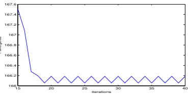
Figure 1 shows a counter-example of the original PNMF algorithm for I-divergence using Eqs. (1), (3), and (4). We have used theGD95 b data set in the experi-ment. It can be seen that the monotonicity of objective evolution is violated in every other loop since the 19th iteration and the optimization is then stuck in an endless fluctuation without a decreasing trend.
1
http://archive.ics.uci.edu/ml/
2
http://www.cise.ufl.edu/research/sparse/matrices/index.html
3
15 20 25 30 35 40 166
166.2 166.4 166.6 166.8 167 167.2 167.4 167.6
iterations
I−divergence
Fig. 1.A counter example showing that the original PNMF algorithm with normal-ization does not monotonically decrease the I-divergence for theGD95 bdata set.
4.2 Training Time Comparison
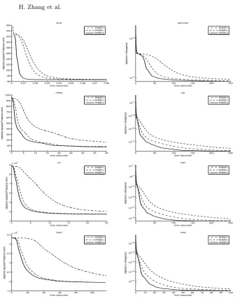
Figure 2 shows the objective evolution curves using the compared methods. One can see that the objectives of the proposed methods, PNMFc and PNMFa, monotonically decrease for the whole iterative learning process without any un-expected rises. Furthermore, PNMFa generally converges the fastest as its curves are below the other two in all plots.
In addition to qualitative analysis, we have also compared the benchmark on converged time of the three methods. Table 2 summarizes the means and standard deviations of the resulting converged time. The converged time is Table 2.The mean (µ) and standard deviation (σ) of the converged time (seconds).
(a) Criterion: the squared Euclidean distance
method wine sonar mfeat orl feret
PNMFn 0.97±0.03 0.97±0.01 26.14±1.54 40.37±1.03 30.80±7.34 PNMFc 0.22±0.11 0.22±0.11 68.57±1.75 117.26±1.74 107.58±24.43 PNMFa 0.06±0.03 0.06±0.03 19.10±0.70 29.89±1.48 19.97±5.60
(b) Criterion: the I-divergence
method worldcities swimmer cisi cran med
PNMFn 8.35±3.71 309.78±8.78 478.43±43.51 438.98±41.71 321.94±34.90 PNMFc 14.07±2.98 613.04±20.63 863.89±69.23 809.61±62.64 566.99±64.44 PNMFa 4.68±1.44 193.47±5.43 193.23±18.70 189.41±18.50 132.67±13.86
calculated as follows. We first find the earliest iteration of PNMFn where the objective Dn is sufficiently close to its minimum D∗
: |Dn −D∗
|/D∗
< 0.001. The corresponding time is recorded as the converged time of the PNMFn. For the PNMFc evolution, the converged time is that of the first iteration where the objectiveDc fulfills|Dc−D∗
|/D∗
0 0.01 0.02 0.03 0.04 0.05 0.06 0.07 0.08
objective (squared Frobenius norm)
wine
objective (squared Frobenius norm)
mfeat
objective (squared Frobenius norm)
orl
objective (squared Frobenius norm)
feret
Fig. 2.Evolutions of objectives using the compared methods based on (left) squared Euclidean distance and (right) I-divergence.
among the three compared: it is 1.5 to 2 times faster than PNMFn and 3 to 5 times faster than PNMFc. The advantage over PNMFn is more significant for the two small data setswine andsonar.
5
Conclusions
multiplicative update rules. Firstly, relaxing the exponent of the multiplying factor to any positive number can lead to theoretically convergent update rules without extra normalization. Secondly, further relaxation by allowing variable exponent can accelerate the iterative learning. Empirical results show that the proposed algorithm not only monotonically decreases the dissimilarity objective but also converges significantly faster than the previous implementation.
The accelerated algorithms facilitate application of the PNMF method. More large-scale datasets will be tested in the future. Moreover, the proposed adaptive exponent technique is readily extended to other fixed-point algorithms that use multiplicative updates.
A
Appendix: Proof of Theorem 1
A.1 The Euclidean distance case
We rewrite the squared Euclidean distance as
DEU(X||WfWfTX) =−2TrWfTXXTWf+X
The first term on the right is upper-bounded by its linear expansion at the current estimateW:
−2TrWfTXXTWf
second term can be upper-bounded by using Jensen’s inequality as follows:
X
We can then construct the auxiliary function
G(W,f W) =−2TrWfTAW
imizing G(Wf,W) is implemented by setting its gradient with respect toWf to zero, which yields the update rule Eq. (5) withη= 1/3.
A.2 The I-divergence case
We rewrite the I-divergence as
The first term is upper-bounded using the Jensen’s inequality: where A is defined in Eq. (3). For the second term, we can rewrite it with B
defined in Eq. (3) and obtain its upper bound with Uike =Wikf andUik=Wik.
We can then construct the auxiliary function
G(W,f W) =−X
1. Cichocki, A., Zdunek, R., Phan, A.H., Amari, S.: Nonnegative Matrix and Tensor Factorizations: Applications to Exploratory Multi-way Data Analysis. John Wiley (2009)
2. Ding, C., Li, T., Jordan, M.: Convex and semi-nonnegative matrix factorizations. IEEE Transactions on Pattern Analysis and Machine Intelligence 32(1), 45–55 (2010)
3. F´evotte, C., Bertin, N., Durrieu, J.L.: Nonnegative matrix factorization with the Itakura-Saito divergence: With application to music analysis. Neural Computation 21(3), 793–830 (2009)
4. Hoyer, P.O.: Non-negative matrix factorization with sparseness constraints. Jour-nal of Machine Learning Research 5, 1457–1469 (2004)
5. Kim, H., Park, H.: Sparse negative matrix factorizations via alternating non-negativity-constrained least squares for microarray data analysis. Bioinformatics 23(12), 1495–1502 (2007)
6. Lee, D.D., Seung, H.S.: Learning the parts of objects by non-negative matrix fac-torization. Nature 401, 788–791 (1999)
7. Xu, W., Liu, X., Gong, Y.: Document clustering based on non-negative matrix fac-torization. In: Proceedings of the 26th annual international ACM SIGIR conference on Research and development in informaion retrieval. pp. 267–273 (2003) 8. Yang, Z., Oja, E.: Unified development of multiplicative algorithms for linear and
quadratic nonnegative matrix factorization. IEEE Transactions on Neural Net-works 22(12), 1878–1891 (2011)
9. Yang, Z., Oja, E.: Linear and nonlinear projective nonnegative matrix factorization. IEEE Transaction on Neural Networks 21(5), 734–749 (2010)