Modeling Systems with Internal State using Evolino
Daan Wierstra
1[email protected]
Faustino J. Gomez
1[email protected]
J ¨urgen Schmidhuber
1,2[email protected]
1 IDSIA, Galleria 2, 6928 Lugano, Switzerland
2 TU Munich, Boltzmannstr. 3, 85748 Garching, M ¨unchen, Germany
ABSTRACT
Existing Recurrent Neural Networks (RNNs) are limited in their ability to model dynamical systems with nonlinearities and hidden internal states. Here we use our general frame-work for sequence learning, EVOlution of recurrent systems with LINear Outputs (Evolino), to discover good RNN hid-den node weights through evolution, while using linear re-gression to compute an optimal linear mapping from hidden state to output. Using the Long Short-Term Memory RNN Architecture, Evolino outperforms previous state-of-the-art methods on several tasks: 1) context-sensitive languages, 2) multiple superimposed sine waves.
Categories and Subject Descriptors
I.2.6 [Artificial Intelligence]: Learning—Connectionism and neural nets
General Terms
Experimentation, Performance, Algorithms
Keywords
Time-series prediction, Recurrent Neural Networks, Evolu-tion and Learning
1.
INTRODUCTION
The kinds of sophisticated behaviors we would like arti-ficial agents to perform in the the future will require them to build predictive models of their environment. For exam-ple, imagine an active-vision-based robot trying to locate an object in a cluttered space. The robot receives a sequence (time-series) of sensory images from which it decides the most profitable place to look next. To solve this task effi-ciently, the robot must anticipate the location of the object based on some kind of short-term memory orinternal state
that helps it determine where it is and where it has been, both spatially and in the sequence sub-goals necessary for
Permission to make digital or hard copies of all or part of this work for personal or classroom use is granted without fee provided that copies are not made or distributed for profit or commercial advantage and that copies bear this notice and the full citation on the first page. To copy otherwise, to republish, to post on servers or to redistribute to lists, requires prior specific permission and/or a fee.
GECCO’05, June 25–29, 2005, Washington, DC, USA.
Copyright 2005 ACM 1-59593-010-8/05/0006 ...$5.00.
accomplishing the task. Otherwise, if the robot does not maintain a useful representation of past experience, it will waste time taking actions that provide no new information about the target object’s likely location.
Artificial neural networks are a popular class of models for making predictions from time-series because they are theo-retically capable of approximating any continuous mapping with arbitrary precision [4]. Normally, networks are trained using gradient descent, but recently evolutionary computa-tion has been used to either evolve the network structure and then learn the weights via gradient descent (e.g. for Multi-Layer perceptrons [25, 5, 13], and Radial Basis Func-tion Networks (RBF) [21]), or to bypass learning altogether by evolving weight values as well [26]. However, because these methods use feedforward architectures, none of them implement generalsequence predictors. That is, predictors that can detect temporal dependencies in the input data that span an arbitrary number of time steps. The Mackey-Glass time-series that is often used to test these methods [21, 25, 3, 5, 13], for instance, can be predicted very accu-rately using a feedforward network with a relatively short time-delay window on the input.
Recurrent Neural Networks (RNNs; [20, 18, 23]) can po-tentially implement general predictors by using feedback connections to maintain internal state. Unfortunately, RNNs are notoriously difficult to train, even using evolution, when the desired network output is a complex function of poten-tially the entire input history. In this paper, we demon-strate a method called EVOlution of recurrent systems with LINear Outputs (Evolino; [19]), for automatically design-ing general sequence predictors. The method combines the evolution of RNNs with analytical methods for computing optimal linear mappings. The approach is demonstrated on two tasks that cannot be solved using a finite set of previous inputs (i.e. using feedforward networks): context-sensitive languages, and superimposed sine wave functions.
The next section provides some background on the state of the art in sequence prediction using recurrent neural net-works. Section 3 outlines the Evolino algorithm and scribes the specific implementation components in more de-tail. Section 4 present our experiments in the two domains described above, and sections 5 and 6 discuss the approach in a broader context and summarize our conclusions.
2.
RECURRENT NEURAL SEQUENCE
PREDICTION
Re-current Learning is only practical when a short time window (less than 10 time-steps) is sufficient to predict the correct system output. For longer temporal dependencies, the gra-dient vanishes as the error signal is propagated back through time so that network weights are never adjusted correctly to account for events far in the past [2, 9].
Echo State Networks (ESNs; [10]) deal with temporal de-pendencies by simply ignoring the gradients associated with hidden neurons. Composed primarily of a large pool of neu-rons (typically hundreds or thousands) with fixed random weights, ESNs are trained by computing a set of weights analytically from the pool to the output units using fast, linear regression. The idea is that with so many random hidden units, the pool is capable of very rich dynamics that just need to be correctly “tapped” by adjusting the output weights. This simple approach is currently the title holder in the Mackey-Glass time-series benchmark, improving on the accuracy of all other methods by as much as three orders of magnitude [10].
The drawback of ESNs, of course, is that the only truly computationally powerful, nonlinear part of the net does not learn at all. This means that on some seemingly simple tasks, such as generating multiple superimposed sine waves, the method fails. According to our experience, it is also not able to solve a simple context-sensitive grammar task [6]. Moreover, because ESNs use such a large number of pro-cessing units, they are prone to overfitting, i.e. poor gener-alization.
One method that adaptsallweights and succeeds in us-ing gradient information to learn long-term dependencies is Long Short-Term Memory (LSTM; [9, 7]). LSTM uses a specialized network architecture that includesmemory cells
that can sustain their internal activation indefinitely. The cells have input and output gates that learn to open and close at appropriate times either to let in new information from outside and change the state of the cell, or to let acti-vation out to potentially affect other cells or the network’s output. The cell structure enables LSTM to use gradient descent to learn dependencies across almost arbitrarily long time spans. However, in cases where gradient information is of little use due to numerous local minima, LSTM becomes less competitive.
An alternative approach to training RNNs is neuroevo-lution [24]. Instead of using a single neural network, the space of network parameters is searched in parallel using evolutionary computation. This approach has been very ef-fective in solving continuous, partially observable reinforce-ment learning tasks where the gradient is not directly avail-able, outperforming conventional methods (e.g. Q-learning, SARSA) on several difficult learning benchmarks [15, 8]. However, neuroevolution is rarely used for supervised learn-ing tasks such as time series prediction because it has diffi-culty fine-tuning solution parameters (e.g. network weights), and because of the prevailing maxim that gradient informa-tion should be used when it is available.
Next we describe the Evolino algorithm, which combines elements of the three methods discussed in this section, to address the disadvantages of each.
3.
THE EVOLINO ALGORITHM
Evolino is a general framework for temporal sequence pre-diction that combines neuroevolution and traditional meth-ods for computing optimal linear mappings, such as linear
Evolino Network Evaluation(net)
Phase 1
resetnet
for eachtraining sequenceu
for eachtime stept
φ(t)←activatenetwith inputu(t)
storeφ(t) in Φ
compute linear mappingW from Φ to targetsD
Phase 2
resetnet error←0
for eachtraining sequenceu
for eachtime stept
φ(t)←activatenetwith inputu(t)
compute outputsy(t)←W φ(t)
error←error+ (y(t)−d(t))2
returnf itness← −error
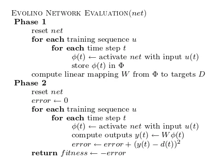
Figure 1: Evolino Network Evaluation. Evolino works are evaluated in two phases. In the first, the net-work is fed the training sequences, and the activation pattern of the network is saved at each time step. At this point the network does not have connections to its outputs with which to make predictions. Once the entire training set has been seen, the output weights are calcu-lated analytically, and the training set is seen again, but now the network produces outputs. The error between these predictions and the correct (target) values is used as a fitness score to be minimized by genetic search.
regression. The underlying principle of Evolino is that often a linear model can account for a large number of properties of a problem. The non-linear properties that are not pre-dicted by the linear model, are then dealt with by evolution. An Evolino network consists of two parts: (1) a non-linear recurrent subnetwork that receives external input, and (2) a linear layer that maps the state of the subnetwork to the output units. The weights of recurrent part of the network are evolved, while the weights of the output layer are com-puted analytically when the recurrent subnetwork is eval-uated during evolution. This procedure generalizes ideas from Maillard [12], in which a similar hybrid approach was used train feedforward networks of radial basis functions.
Network evaluation proceeds in two phases (figure 1). In the first phase, a training set of sequences obtained from the system, {ui, di}, i = 1..k, each of length li, is presented to the network. For each sequenceui, starting at timet= 0, each input patternui(t) is successively propagated through the recurrent subnetwork to produce a vector φi(t) that is stored in an×Pk
i l
imatrix Φ. Associated with each
φi(t), is atargetvectordiinDcontaining the correct output values for each time step. Once allksequences have been seen, the output weightsWare computed using linear regression from Φ toD. The vectors in Φ (i.e. the values of each of then
outputs over the entire training set) form a non-orthogonal basis that is combined linearly byW to approximateD.
ESP
LSTM Network
output input
pseudo−inverse
weights
Time series
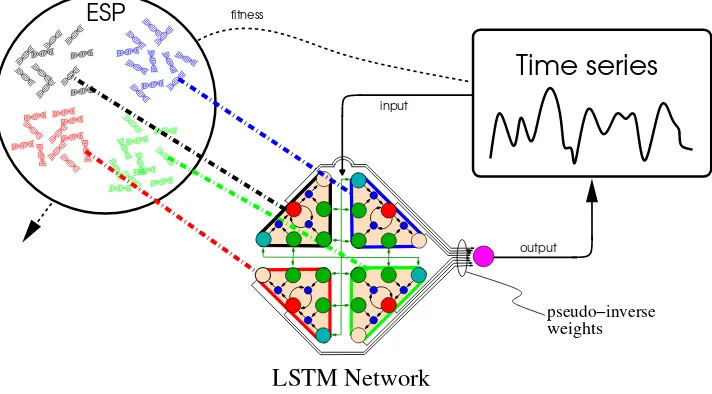
fitnessFigure 2: Enforced SubPopulations (ESP). ESP evolves neurons instead of full networks. Neurons are segregated into subpopulations, and networks are formed by randomly selecting one neuron from each subpopulation. A neuron accumulates a fitness score by adding the fitness of each network in which it participated. The best neurons within each subpopulation are mated to form new neurons. The network shown here is an LSTM network with four memory cells. In Evolino, only the connection weights in the recurrent part of the network are evolved. The weights to the output units are computed analytically during each evaluation.
Neuroevolution is normally applied to reinforcement learn-ing tasks where correct network outputs (i.e. targets) are not knowna priori. Here we use neuroevolution for supervised learning to circumvent the problem of vanishing gradient. In order to obtain the precision required for time-series tion, we do not try to evolve a network that makes predic-tions directly. Instead, the network outputs a set of vectors that form a basis for linear regression. The intuition is that finding a sufficiently good basis is easier than trying to find a network that models the system accurately on its own.
The next sections describe the particular instantiation of Evolino used in this study.
3.1
Enforced SubPopulations
Enforced SubPopulations differs from standard neuroevo-lution methods in that instead of evolving complete net-works, itcoevolvesseparate subpopulations of network com-ponents orneurons (figure 2). Evolution in ESP proceeds as follows:
1. Initialization. The number of hidden units H in the networks that will be evolved is specified and a subpop-ulation of n neuron chromosomes is created for each hidden unit. Each chromosome encodes a neuron’s in-put, outin-put, and recurrent connection weights with a string of random real numbers.
2. Evaluation. A neuron is selected at random from each of theH subpopulations, and combined to form a re-current network. The network is evaluated on the task and awarded a fitness score. The score is added to the
cumulative fitnessof each neuron that participated in the network.
3. Recombination. For each subpopulation the neurons are ranked by fitness, and the top quartile is recom-bined using 1-point crossover and mutated using Cauchy
distributed noise to create new neurons that replace the lowest-ranking half of the subpopulation.
4. Repeat the Evaluation–Recombination cycle until a sufficiently fit network is found.
ESP searches the space of networks indirectly by sampling the possible networks that can be constructed from the sub-populations of neurons. Network evaluations serve to pro-vide a fitness statistic that is used to produce better neurons that can eventually be combined to form a successful net-work. This cooperative coevolutionary approach is an exten-sion to Symbiotic, Adaptive Neuroevolution (SANE; [15]) which also evolves neurons, but in a single population. By using separate subpopulations, ESP accelerates the special-ization of neurons into different sub-functions needed to form good networks because members of different evolving sub-function types are prevented from mating. Subpopula-tions also reduce noise in the neuron fitness measure because each evolving neuron type is guaranteed to be represented in every network that is formed. This allows ESP to evolve recurrent networks, where SANE could not.
Σ
Σ
G
FG
FG
IG
Io
G
G
o
S
S
O
O
Figure 3: Long Short-Term Memory. The figure shows an LSTM network with one external input (lower-most
circle), one output (uppermost circle), and twomemory
cells(two triangular regions). Each cell has an internal
stateStogether with a forget gate (GF) that determines
how much the state is attenuated at each time step. The
input gate (GI) controls access to the state by the
ex-ternal inputs and the output of other cells which are
summed into eachΣunit, and the output gate (GO)
con-trols when and how much the cell fires. Small dark nodes represent the multiplication function.
need to be changed radically. To ensure that most changes are small while allowing for larger changes to some weights, ESP uses the Cauchy distribution to generate noise:
f(x) = α
π(α2+
x2) (1)
With this distribution 50% of the values will fall within the interval±αand 99.9% within the interval 318.3±α. This technique of “recharging” the subpopulations keeps diversity in the population so that ESP can continue to make progress toward a solution even in prolonged evolution.
Burst mutation is similar to the Delta-Coding technique of Whitley [22] which was developed to improve the precision of genetic algorithms for numerical optimization problems.
3.2
Long Short-Term Memory
LSTM is a recurrent neural network purposely designed to learn long-term dependencies via gradient descent. The unique feature of the LSTM architecture is thememory cell
that is capable of maintaining its activation indefinitely (fig-ure 3). Memory cells consist of a linear unit which holds the
stateof the cell, and three gates that can open or close over time. The input gate “protects” a neuron from its input: only when the gate is open, can inputs affect the internal state of the neuron. The output gate lets the internal state out to other parts of the network, and the forget gate enables the state to “leak” activity when it is no longer useful. The gates also receive inputs from neurons, and a function over their input (usually the sigmoid function) decides whether they open or close.
The amount each gategiof memory celliis open or closed at timetis calculated by:
gini (t) =σ(
X
j
winijcj(t−1) +
X
k
winikuk(t)), (2)
gf orgeti (t) =σ(X j
wf orgetij cj(t−1) +X k
wf orgetik uk(t)),(3)
giout(t) =σ(
X
j
woutij cj(t−1) +
X
k
woutik uk(t)). (4)
wherew{in,out,f orget}ij is the weight from the outputcjof cell
jto gatei,w{in,out,f orget}ik is the weight from external input
uk to the gatei, andσis the standard sigmoid function. The external inputs to the cell (indicated by the Σs in figure 3) are added up inneti(t):
neti(t) =h(X j
wcellij cj(t−1) +
X
k
wcellik uk(t)), (5)
wherehis usually the identity function. The internal state of celliis:
si(t) =neti(t)giin(t) +gif orget(t)si(t−1), (6)
and the output gates control the cell outputs ci which is squashed by thetanhfunction:
ci(t) =tanh(gouti (t)si(t)). (7)
3.3
Combining ESP and LSTM in Evolino
We apply our general Evolino framework to the LSTM ar-chitecture, using ESP for evolution and regression for com-puting linear mappings from hidden state to outputs. ESP coevolves subpopulations of memory cells instead of stan-dard recurrent neurons (figure 2). Each chromosome is a string containing the external input weights and the input, output, and forget gate weights, for a total of 4∗(I+H) weights in each memory cell chromosome, where I is the number of external inputs andH is the number of memory cells in the network. There are four sets ofI+H weights because the three gates (equations 2, 3, and 4) and the cell itself (equation 5) receive input from outside the cell and the other cells. Figure 4 shows how the memory cells are encoded in an ESP chromosome. Each chromosome in a subpopulation encodes the connection weights for a cell’s input, output, and forget gates, and external inputs.ESP, as described in section 3.1, normally uses crossover to recombine neurons. However, for the present Evolino variant, where fine local search is desirable, ESP uses only mutation. The top quarter of the chromosomes in each sub-population are duplicated and the copies are mutated by adding Cauchy noise (equation 1) to all of their weight val-ues.
The linear regression method used to compute the output weightsWis the Moore-Penrose pseudo-inverse method [17], which is both fast and optimal in the sense that it minimizes the summed squared error. For LSTM networks, the vector
external inputs
output gate
input gate
forget gate
Genotype
Phenotype
Σ
o
G
I
G
F
S
G
O
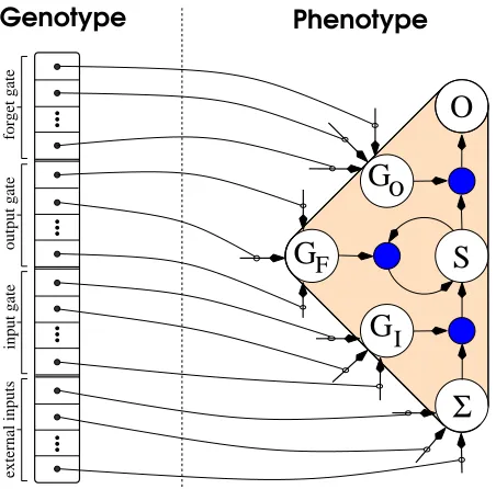
Figure 4: Genotype-Phenotype mapping. Each chromo-some (genotype, left) in a subpopulation encodes the ex-ternal input, and input, output, and forget gate weights of an LSTM memory cell (right). The weights leading out of the state (S) and output (O) units in figure 3 are not encoded in the genotype, but are instead computed at evaluation time by linear regression.
interior of the cells. The output of the network is then:
yi(t) =X j
cj(t)wijstandard+
X
k
sk(t)wikpeephole.
For continuous function generation,backprojectionis used where the predicted outputs are fed back as inputs in the next time step. During training, the correct target values are backprojected, in effect “clamping” the network’s outputs to the right values. During testing, the network backprojects its own predictions. This technique is also used by ESNs, but whereas ESNs do not change the backprojection connec-tion weights, Evolino evolves them, treating them like any other input to the network. In the experiments described below, backprojection was found useful for continuous func-tion generafunc-tion tasks, but interferes to some extent with performance in the discrete context-sensitive language task.
4.
EXPERIMENTAL RESULTS
We carried out experiments on two very different domains: continuous function generation and context-sensitive lan-guages. This choice was made to ensure that Evolino did not only perform well in continuous time series prediction, but also on discrete tasks, since many real world applications have both discrete and continuous elements.
To demonstrate the generality of Evolino, we used exactly the same parameters for both tasks, despite their very dif-ferent characteristics. A bias was added to the forget gates and output gates: +1.5 for the forget gates and −1.5 to the output gates. This did not affect the overall results of the experiments, but sped up learning, especially dur-ing the first few generations. The initial weights for the
time steps
cell 3
0 500 1000 1500 2000
0 500 1000 1500 2000 2500 −1000
cell 4 cell 2 cell 1
−500
Figure 5: Internal state activations. The state activa-tions for the 4 memory cells of an Evolino network being
presented the stringa800b800c800
. The plot clearly shows how some units function as “counters,” recording how
manyas and bs have been seen.
memory cells were chosen at random from [−0.1,0.1], and the Cauchy noise parameter αboth for recombination and burst mutation was set to 0.00001.
The only difference between the experimental settings of both experiments was the use of backprojection for the su-perimposed sine wave task. Again, adding backprojection to the language task only slows down evolution but does not qualitatively produce worse results.
4.1
Context-Sensitive Grammars
Context-sensitive languages are languages that cannot be recognized by deterministic finite-state automata, and are therefore more complex in some respects than regular lan-guages. In general, determining whether a string of symbols belongs to a context-sensitive language requires remember-ing all the symbols in the strremember-ing seen so far, which rules out the use of non-recurrent neural architectures. To compare Evolino-based LSTM with published results for Gradient-based LSTM [6], we chose the language anbncn.
The task was implemented using networks with 4 input units, one for each symbol (a, b, c) plus the start symbolS, and four output units, one for each symbol plus the termina-tion symbol T. Symbol strings were presented sequentially to the network, with each symbol’s corresponding input unit set to 1, and the other three set to -1. At each time step, the network must predict the possible symbols that could come next in a legal string. Legal strings in anbncn are those in which the number ofas,bs, andcs is equal, e.g.ST,SabcT,
SaabbccT,SaaabbbcccT, and so forth. So, forn= 3, the set of input and target values would be:
Input: S a a a b b b c c c
Target: a/T a/b a/b a/b b b c c c T
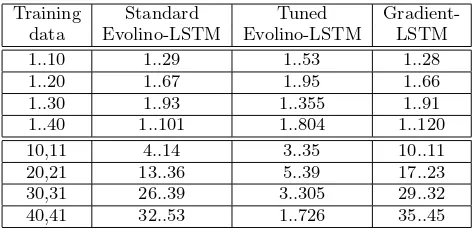
Evolino-based LSTM networks were evolved using 8 dif-ferent training sets, each containing legal strings with values fornas shown in the first column of table 1. In the first four sets,nranges from 1 tok, wherek= 10,20,30,40. The sec-ond four sets consist of just two training samples, and were intended to test how well the methods could induce the lan-guage from a nearly minimal number of examples.
re-Training Standard Tuned
Gradient-data Evolino-LSTM Evolino-LSTM LSTM
1..10 1..29 1..53 1..28
1..20 1..67 1..95 1..66
1..30 1..93 1..355 1..91
1..40 1..101 1..804 1..120
10,11 4..14 3..35 10..11
20,21 13..36 5..39 17..23
30,31 26..39 3..305 29..32
40,41 32..53 1..726 35..45
Table 1: Results for the anbncn language. The ta-ble compares Evolino-based LSTM with Gradient-based
LSTM on the anbncn language task. “Standard” refers
to Evolino with the parameter settings used for both
dis-crete and continuous domains (anbncnand superimposed
sine waves). The “Tuned” version is biased to the lan-guage task: we additionally squash the cell input with
the tanh function. The leftmost column shows the set
of strings used for training in each of the experiments. The other three columns show the set of legal strings to which each method could generalize after 50 genera-tions (3000 evaluagenera-tions), averaged over 20 runs. The up-per training sets contain all strings up to the indicated length. The lower training sets only contain a single pair. Evolino-based LSTM generalizes better than Gradient-based LSTM, most notably when trained on only two ex-amples of correct behavior. The Gradient-based LSTM results are taken from [6].
sults with those of Gradient-based LSTM from [6]. “Stan-dard Evolino” uses parameter settings that are a compro-mise between discrete and continuous domains. If we set
h in equation 5 to the tanh function, we obtain “Tuned Evolino.”
The Standard Evolino networks had generalization very similar to that of Gradient-based LSTM on the 1..k train-ing sets, but slightly better on the two-example traintrain-ing sets. Tuned Evolino showed a dramatic improvement over Gradient-based LSTM on all of the training sets, but, most remarkably on the two-example sets where it was able to generalize on average to all strings up ton= 726 after being trained on onlyn={40,41}. Figure 5, shows the internal states of each of the 4 memory cells of one of the evolved networks while processinga800
b800
c800 .
4.2
Multiple Superimposed Sine Waves
Learning to generate a sinusoidal signal is a relatively sim-ple task that requires only one bit of memory to indicate whether the current network output is greater or less than the previous output. When sine waves with frequencies that are not integer multiples of each other are superimposed, the resulting signal becomes much harder to predict because its wavelength can be extremely long, i.e. there are large num-ber of time steps before the periodic signal repeats. Gen-erating such a signal accurately without recurrency would require a prohibitively large time-delay window using a feed-forward architecture.Jaeger reports [11] that Echo State Networks are unable to learn functions composed of even two superimposed os-cillators, in particularsin(0.2x) +sin(0.311x). The reason for this is that the dynamics of all the neurons in the ESN
No. sines No. cells Training error Gen. error
2 10 0.0008 0.0034
3 15 0.0018 0.0195
4 20 0.0893 4.73
5 20 0.125 13.4
Table 2: Results for multiple superimposed sine waves. The table shows the number of memory cells, training error, and generalization error for each of the superim-posed sine wave functions. The training error is the sum
of squares error on time steps100to400(i.e. the washout
time is not included in the measure). The generalization
error is calculated for time steps 400 to700. The error
values are the average over 20 experiments.
“pool” are coupled, while this task requires that the two underlying oscillators be represented independently by the network’s internal state.
Here we show how Evolino-based LSTM not only can solve the two-sine function mentioned above, but also more complex functions formed by adding up to three more sine waves. The following table shows the four functions used in our experiments, starting with the two-sine suggested by Jaeger [11]. Each of the functions we used was construct byPn
i=1sin(λix), wherenis the number of sine waves and
λ1= 0.2, λ2= 0.311, λ3= 0.42, λ4= 0.51, andλ5= 0.74. Evolino used the same parameter settings as in the pre-vious section, except that backprojection was used (see sec-tion 3.3). Networks were evolved to predict, without any external input, the first 400 time steps of each function, us-ing a “washout time” of 100 steps. Durus-ing the washout time the vectorsφ(t) are not collected for calculating the pseudo-inverse. After a specified number of generations, the best networks were then tested for generalization on data points from time-steps 400..700. The first three tasks, n= 2,3,4, used subpopulations of size 40 and simulations were run for 50 generations. The five-sine wave task,n= 5, proved much more difficult to learn requiring a larger subpopulation size of 100, and simulations were allowed to run for 150 genera-tions.
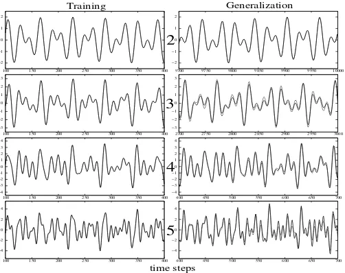
Table 2 shows the number of memory cells used for each task, and the average error on both the training set and the testing set for the best network found during each evolution-ary run. Figure 6 shows the behavior of one the successful networks from each of the tasks. The column on the left shows the target signal from Table 2, and the output gen-erated by the network on the training set. The column on the right shows the same curves forward in time to show the generalization capability of the networks. For the two-sine function, even after 9000 time-step, the network continues to generated the signal accurately. As more sines are added, the prediction error grows more quickly, but the overall be-havior of the signal is still retained, showing that the net-work has succeeded in representing the signal’s underlying attractors.
5.
DISCUSSION
el-5
Training
time steps
Generalization
4
3
2
−4
250 300 350 400 −4
−3 −2 −1 0 1 2 3 4
100 150 200 250 300 350 400 −3
−2 −1 0 1 2 3
100 150 200 250 300 350 400
−4 −3 −2 −1 0 1 2 3 4
400 450 500 550 600 650 700 −3
−2 −1 0 1 2 3
2700 2750 2800 2850 2900 2950 3000
−4 −2 0 2 4
400 450 500 550 600 650 700 −2
−1 0 1 2
100 150 200 250 300 350 400 −2 −1 0 1 2
9700 9750 9800 9850 9900 9950 10000
150 100
4 2 0 −2
200
Figure 6: Performance of Evolino-based LSTM on the superimposed sine wave tasks. The plots show the behavior of a typical network produced after a specified number of generations: 50 for the two-, three-, and four-sine functions, and 150 for the five-sine function. The first 300 steps of each function, in the left column, were used for training. The curves in the right column show values predicted by the networks (dashed curves) further into the future vs. the corresponding reference signal (solid curves). While the onset of noticeable prediction error occurs earlier as more sines are added, the networks still track the correct behavior for hundreds of time steps, even for the five-sine function.
ements in the series that can be far in past. This general ability to base decisions on past experience is essential for building robust anticipatory systems that can function in uncertain real-world environments.
On the context-sensitive grammar task, Evolino outper-formed Gradient-based LSTM—the only RNN architecture previously able to learn this task. And, it was able capture the underlying dynamics of up to five superimposed sine waves, while Echo State Networks are unable to cope with even the two-sine case. The very different nature of these two tasks suggests that Evolino could be widely applicable to modeling complex processes, such as speech, that have both discrete and continuous properties.
Although Evolino does not use learning in the traditional gradient-descent sense, it is related to other hybrid evolu-tionary methods that adapt weight values during interaction
with the evaluation environment [16, 25, 14]. The “on the fly” computation of the output layer can be viewed as a kind of learning, and, like learning, it effectively distorts the fitness landscape in a Baldwinian sense [1].
The version Evolino used in this paper is but one possi-ble instantiation of the general framework. Many others are possible. For instance, ESP could be replaced by a neuroevo-lution method that evolves topology as well, or the genetic search, in general, could be complemented by local search, or even gradient-descent. Also, other network architectures could be evolved, such as Higher-Order networks.
but also to accelerate the evolution of robot controllers. An Evolino-based model that captures the dynamic elements of an environment that are salient for a particular robot task, can serve as a computationally efficient surrogate for the real-world in which to evaluate candidate controllers.
6.
CONCLUSION
In this paper, we demonstrated an implementation of EVO-lution of recurrent systems with LINear Outputs (Evolino) that used the Enforced SubPopulations neuroevolution algo-rithm to coevolve Long Short-Term Memory cells. The ap-proach was evaluated on two different prediction tasks that require short-term memory: a discrete problem, context-sensitive languages, and a continuous time-series, multiple superimposed sine waves. In both cases, our results im-proved upon the state of the art, demonstrating that the method is a powerful and general sequence prediction strat-egy.
Acknowledgments
This research was partially funded by CSEM Alpnach and the EU MindRaces project, FP6 511931.
7.
REFERENCES
[1] J. M. Baldwin. A new factor in evolution.The American Naturalist, 30:441–451, 536–553, 1896. [2] Y. Bengio, P. Simard, and P. Frasconi. Learning long-term dependencies with gradient descent is difficult.IEEE Transactions on Neural Networks, 5(2):157–166, 1994.
[3] S. Chen. Combined genetic algorithm optimization and regularized orthogonal least squares learning for radial basis function networks.IEEE Transactions on Neural Networks, 10(5), September 1999.
[4] G. Cybenko. Approximation by superpositions of a sigmoidal function.Mathematics of Control, Signals, and Systems, 2:303–314, 1989.
[5] I. D. Falco, A. Iazzetta, P. Natale, and E. Tarantino. Evolutionary neural networks for nonlinear dynamics modeling. InParallel Problem Solving from Nature 98, volume 1498 ofLectures Notes in Computer Science, pages 593–602, 1998.
[6] F. A. Gers and J. Schmidhuber. LSTM recurrent networks learn simple context free and context sensitive languages.IEEE Transactions on Neural Networks, 12(6):1333–1340, 2001.
[7] F. A. Gers, J. Schmidhuber, and F. Cummins. Learning to forget: Continual prediction with LSTM.
Neural Computation, 12(10):2451–2471, 2000. [8] F. Gomez and R. Miikkulainen. Solving
non-Markovian control tasks with neuroevolution. In
Proceedings of the 16th International Joint Conference on Artificial Intelligence, Denver, CO, 1999. Morgan Kaufmann.
[9] S. Hochreiter and J. Schmidhuber. Long short-term memory.Neural Computation, 9(8):1735–1780, 1997. [10] H. Jaeger. Harnessing nonlinearity: Predicting chaotic
systems and saving energy in wireless communication.
Science, 304:78–80, 2004.
[11] H. Jaeger. http://www.faculty.iu-bremen.de/
hjaeger/courses/seminarspring04/esnstandardslides.pdf, 2004.
[12] E. P. Maillard and D. Gueriot. RBF neural network, basis functions and genetic algorithms. InIEEE International Conference on Neural Networks, pages 2187–2190, Piscataway, NJ, 1997. IEEE.
[13] H. A. Mayer and R. Schwaiger. Evolutionary and coevolutionary approaches to time series prediction using generalized multi-layer perceptrons. InCongress on Evolutionary Computation, Washington D.C., July 1999.
[14] P. McQuesten and R. Miikkulainen. Culling and teaching in neuro-evolution. In T. B¨ack, editor,
Proceedings of the Seventh International Conference on Genetic Algorithms (ICGA-97, East Lansing, MI), pages 760–767. San Francisco, CA: Morgan
Kaufmann, 1997.
[15] D. E. Moriarty and R. Miikkulainen. Efficient reinforcement learning through symbiotic evolution.
Machine Learning, 22:11–32, 1996.
[16] S. Nolfi, J. L. Elman, and D. Parisi. Learning and evolution in neural networks. Adaptive Behavior, 2:5–28, 1994.
[17] R. Penrose. A generalized inverse for matrices. In
Proceedings of the Cambridge Philosophy Society, volume 51, pages 406–413, 1955.
[18] A. J. Robinson and F. Fallside. The utility driven dynamic error propagation network. Technical Report CUED/F-INFENG/TR.1, Cambridge University Engineering Department, 1987.
[19] J. Schmidhuber, D. Wierstra, and F. Gomez. Evolino: Hybrid neuroevolution/optimal linear search for sequence learning. InProceedings of the 19th International Joint Conference on Artificial Intelligence, 2005.
[20] P. Werbos. Backpropagation through time: what does it do and how to do it. InProceedings of IEEE, volume 78, pages 1550–1560, 1990.
[21] B. Whitehead and T. D. Choate.
Cooperative-Competitive genetic evolution of radial basis function centers and widths for time series prediction. IEEE Transactions on Neural Networks, 7(4):869–880, 1996.
[22] D. Whitley, K. Mathias, and P. Fitzhorn.
Delta-Coding: An iterative search strategy for genetic algorithms. In R. K. Belew and L. B. Booker, editors,
Proceedings of the Fourth International Conference on Genetic Algorithms, pages 77–84. San Francisco, CA: Morgan Kaufmann, 1991.
[23] R. J. Williams and D. Zipser. A learning algorithm for continually running fully recurrent networks.Neural Computation, 1(2):270–280, 1989.
[24] X. Yao. Evolving artificial neural networks.
Proceedings of the IEEE, 87(9):1423–1447, 1999. [25] X. Yao and Y. Liu. A new evolutionary system for
evolving artificial neural networks.IEEE Transactions on Neural Networks, 8(3):694–713, May 1997.
[26] B.-T. Zhang, P. Ohm, and H. Mhlenbein. Evolutionary induction of sparse neural trees.