AN AUTOMATIC ALGORITHM FOR MINIMIZING ANOMALIES AND
DISCREPANCIES IN POINT CLOUDS ACQUIRED BY LASER SCANNING TECHNIQUE
Fabiane Bordina, Luiz Gonzaga Jra b, Fabricio Galhardo Mullera∗, Mauricio Roberto Veroneza c, Marco Scaionid
a
Advanced Visualization Laboratory (VIZLab), University of Vale do Rio dos Sinos (UNISINOS) S˜ao Leopoldo, Brazil - [email protected] - [email protected]
b
Graduate Program in Applied Computing (PIPCA), University of Vale do Rio dos Sinos (UNISINOS) S˜ao Leopoldo, Brazil - [email protected]
c Graduate Program in Geology (PPGEO), University of Vale doRio dos Sinos (UNISINOS)
S˜ao Leopoldo, Brazil - [email protected] d
Department of Architecture, Built Environment and Construction Engineering, Politecnico di Milano Milano, Italy - [email protected]
Commission V, WG V/5
KEY WORDS:Laser Scanning, LiDAR, Remote Sensing, Point Cloud, Return Intensity, Edge Effect, Quadtree, Clustering
ABSTRACT:
Laser scanning technique from airborne and land platforms has been largely used for collecting 3D data in large volumes in the field of geosciences. Furthermore, the laser pulse intensity has been widely exploited to analyze and classify rocks and biomass, and for carbon storage estimation. In general, a laser beam is emitted, collides with targets and only a percentage of emitted beam returns according to intrinsic properties of each target. Also, due interferences and partial collisions, the laser return intensity can be incorrect, introducing serious errors in classification and/or estimation processes. To address this problem and avoid misclassification and estimation errors, we have proposed a new algorithm to correct return intensity for laser scanning sensors. Different case studies have been used to evaluate and validated proposed approach.
1. INTRODUCTION
Laser scanning technique from airborne and ground platforms has been largely used for the reconstruction of high-resolution 3-D to-pography in the field of geosciences and other applications (Shan and Toth, 2008) (Laefer et al., 2014) (Bordin et al., 2013) (Ehlert and Heisig, 2013) (Sahin et al., 2012) (Buckley et al., 2008). The capture of spatial data through a laser scanner has become pop-ular due the difficulties to access some targets or part of them, and mainly by the capability for reconstructing high accurate 3D models. Besides, the equipment can scan thousands of points per second (Burton et al., 2011) that reduces the field time. Further-more, using digital data, it’s possible to make the analysis in the office or laboratory, which reduces the fieldwork cost, time and in the most cases, human risks.
The digital acquisition by laser scanning records not only the tar-get’s position and color, but also the return intensity of the laser pulse. In the latest years, the reflection strength of the laser pulse intensity which returns to the sensor, or simply return intensity, has been also exploited to analyze and classify rock properties and for biomass and carbon storage estimation. However, anoma-lies and discrepances can occur during the remote sensing, mainly the edge effect. The edge effect may occur when the laser collides partially with the target and part of the signal is lost or, also, col-lides with other undesired objects in the background. This effect makes the laser’s return intensity be incorrect. When the purpose of the application is to analyze the reflectance of the laser’s re-turn intensity to exploit properties of materials that compose the target, the edge effect should be compensated to avoid misclassi-fication errors.
To address this important problem, we have proposed a new algo-rithm to recover the correct returned laser intensity when an edge
∗Thanks to CAPES and FINEP agencies for funding
effect is detected in collected data by laser scanning sensors. The methodology approaches mainly three different parameters: the intensity for each returned pulse, the laser scanners position, and the beams divergence. The algorithm core is based on point-cloud clustering, when each group corresponds to a different material. When the edge effect appears, those points which were affected are grouped into a class (existing or new). Under presence of the edge effect, one of the groups is tagged as edge effect group and the intensity value in this group needs to be corrected. Then, to determine the correct intensity of the returned pulse, and then to minimize the border effect, the algorithm estimates the collision percentage of the laser pulse with the target and the amount of the returned beam back to the laser station.
Three different case studies have been planned to demonstrate proposed algorithm effectiveness, based on three different tar-gets: (1) artificial, but controlled target; (2) rock target; and (3) a forestry target. The results show that the proposed algorithm for edge-effect compensation is a feasible solution to recover the cor-rect lasers return intensity according to the reflectance of the tar-get structure, providing significant improvements and promising results for the development of applications based on laser scan-ning technique for different applications, including geoscience, civil engineering, environmental and geological studies.
2. ANOMALIES E DISCREPANCIES ON POINT CLOUDS
are associated to 3D-points. Finally, each point on point cloud has the following attributes(X, Y, Z, R, G, B, i), where(X, Y, Z)
represents 3D point coordinates, its respective colour(R, G, B)
obtained from images and finally the return intensity.
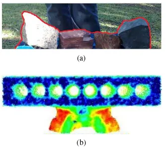
We mean by edge (or border), the target silhouette where the laser’s beam stop colliding with the target and start to collide with the background or a percentage of the laser beam is lost. ure 1.(a) shows the rock’s edges delimited by a red contour. Fig-ure 1.(b) shows controlled target, with edges delimited by green contours.
(a)
(b)
Figure 1: (a) The red area is the edge of the target where edge effect may appear. (b) The green points inside the circles and around the blue rectangle represent the edge effect seen in the 3D point cloud.
The intensity data (i) is directly proportional to the target’s re-flectance and inversely proportional to the target’s distance, and suffer influences of atmospheric conditions and other agents (Ahokas et al., 2006) (H¨ofle and Pfeifer, 2007). The greater is the distance from the laser scanner to the target, the wider and less intense the laser pulse will be. The atmospheric conditions like the presence of rain also can modify the intensity data (Hodgetts, 2013). In general, a wider and less intense laser pulse due to the distance or weather results in an intensity data that does not correspond to the target’s material. There are works which propose to correct the intensity data on the basis of the distance sensor−target (H¨ofle and Pfeifer, 2007) (Kaasalainen et al., 2011) and, also, applied in geological researches (Burton et al., 2011) as a remote sensing technique for rock properties analysis (Hodgetts, 2013).
Pingbo et al (Tang et al., 2009) also have proposed a method for estimating edge loss in laser scanned data by considering the im-pacts of scanning distance, density of data and incidence angle on the edge loss. The proposed method explores the return intensity, laser scanner’s position and signals divergence, on the estimation algorithm, and a couple of controlled are performed to show the algorithm effectiveness. We have considered similar parameters to perform estimation and on corrected points recovering.
3. THE PROPOSED ALGORITHM
By using clustering algorithms, the point cloud can by classified into different groups based on the intensity data. Each group cor-responds to one different material. Because the existence of the edge effect, one of the groups is going to be the edge effect group. The intensity value in the last group needs to be recovered. In the Figure 2, each color from the point cloud belongs to a different group of intensity.
Figure 2: In the upper part four blocks scanned for the second experiments are shown. In the lower part, the effect of clustering intensity data is depicted.
On algorithm development, we have assumed the relation be-tween the return intensity and the percentage of the collision is linear. So it can be defined by the equation 1 as the intensity re-covery formula, to be applied to the edge effect clustered group.
Ir= Im
ce (1)
whereIr is the recovered intensity value,Im is the measured intensity by the laser and thece is the estimated collision value of the laser pulse with its target, where{ce∈R; 0< ce≤1}.
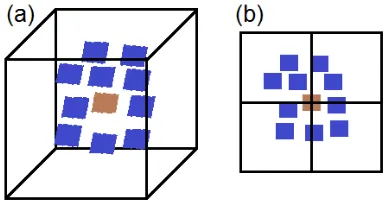
Once the ce value is defined, it’s easy to calculate the correct intensity value. Let’s considerP as the set of clustered points which belong to the edge effect group,Qthe set of all points that belong to the entire point cloud,pis a point from the setP being analysed andqis a point from the setQ. For each point pthat belongs to P, an axis-aligned bounding box (AABB) is created centered inp. All points q from the set Q are tested to verify if qis inside the AABB box. The AABB size is de-fined through the spacing between points, which generates the spacingvariable. This can be computed based on the scanning configuration because it’s necessary to have a minimum number of points to calculate the collision approximation. If theqpoint is inside the AABB, thenqis inserted in a quadtree ofnlevel cre-ated in the same AABB’s position and with same AABB’s size. Figure 3 shows the AABB centered on the pointpwith neighbor-hood points and also shows the quadtree positioned in the pointp (the point being analysed) with the points around.
Figure 3: Subfigure (a) shows the AABB bounding box with the points inside. (b) Shows the quadtree centered in the same place of the AABB with points split in different cells.
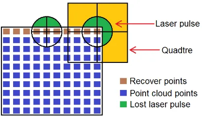
perc= 1
4n (2)
whereperc is the total collision percentage for each quadtree quadrant andnis the quadtree level.
Algorithm 1Laser intensity recovery algorithm
Require: P = {p1, p2, . . . , pn}, Q =
{q1, q2, . . . , qm}, n, spacing
1: for allp∈Pdo
2: aabb←CreateAABB(p.x, p.y, p.z, spacing)
3: quadtree←CreateQuadtree(p.x, p.y, p.z, spacing)
4: for allq∈Qdo
5: ifq⊂aabbthen
6: quadtree←q 7: end if
8: end for
9: quads←Sort(quadtree, n)
10: highest←quads[0]
11: percP erQuad←100 4n
12: sum= 0
13: for allquad∈quadsdo
14: sum+ = (quad∗percP erQuad)
highest 15: end for
16: sum= sum
100
17: p.intensity=p.intensity sum 18: end for
In the worst case scenario, the algorithm has numerical burden ofO(n2), where the most part of the points from the point cloud are clustered and considered belonging to the edge effect group. Also, to determine the collision percentage is required to go through all the point cloud testing if each point is inside the AABB Bound-ing Box.
4. RESULTS AND DISCUSSION
The proposed algorithm has been evaluated to correct the return intensity signal on the occurrence of the edge effect for three dif-ferent case studies : (1) synthetic point cloud, (2) rock’s classifi-cation and (3) forestry target.
4.1 Case Study I: synthetic point cloud
For the first study, it was created a synthetic point cloud where all the points, with one line exception, have the intensity value of 100, over a normalized range between 0-255. The ”edge effect” line is the sequence of points in a straight line which has intensity
value of 50. This point cloud was clustered and the points were separated into two groups. Figure 4 shows the synthetic point cloud before and after the recovery algorithm. In Figure 4(a), there are two groups, the blue points correspond to the correct intensity value while the gray ones correspond to the edge effect group. The red line highlights the edge effect points. After apply-ing the intensity recovery algorithm in the synthetic point cloud and clustering that point cloud again, almost all the points have been assigned to the same group. Figure 4(b) shows almost all the points in the same group and the red line highlight the points which were part of the edge effect and now is part of the same group. Since the synthetic point cloud has few points, its data is detailed in the table 1.
Figure 4: Synthetic point cloud clustered before the intensity covery (a). Synthetic point cloud clustered after the intensity re-covery (b).
Table 1: Intensity data recovered through the created algorithm
Original Collision Recovered Difference (100)
50 30.8642% 162 62
50 34.7222% 144 44
50 34.7222% 144 44
50 46.2963% 108 8
50 55.5555% 90 10
50 50.9259% 98 2
50 43.6508% 114 14
50 39.6825% 126 26
50 30.8642% 162 62
50 30.5555% 163 63
It’s noticeable that the points in corners of the point cloud fea-ture worst results than the points in the center of the point cloud. This fact occurs because the synthetic point cloud ends abruptly in the corners. While it does not happen in the point clouds of real objects captured by laser scanning. Indeed, in such case, the points in the corners would not have the same intensity value of the points in the center. Figure 5 shows why the recovered in-tensity differences occur. But the collision estimation is valid, since the collision percentage for corner points are smaller than the collision estimation of the points in the center.
4.2 Case Study II: rock’s classification
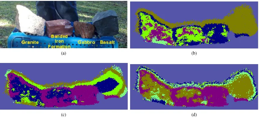
The second evaluation, it was used a real point cloud scanned with TLS - Optech ILRIS-3D1. Different types of rock blocks were put in a basement to be scanned with the TLS ILRIS-3D. Figure 2 shows that after clustering the point cloud, one intensity group is clearly the edge effect.
It’s also possible to see that one rock is part of the edge effect since this specific rock reflects low laser pulse intensity. The Figure 6a shows original target. After applying the algorithm to
1http://www.teledyneoptech.com/index.php/product/
Figure 5: The green area is the lost part of the laser pulse that was estimated correctly by the quadtree, but the synthetic intensity value generated was equal to all points.
correct the intensity data it’s still possible to see a residual edge effect, but smaller than the one int the original point cloud (Fig-ures 6c and 6d). Moreover, it’s possible to distinguish the rock that was masked by the edge effect. The difference of the edges in the Figures 6c and 6d occurs because of the different parameters of the algorithm, but both parameters recovered the intensities of the original point cloud.
These parameters make the AABB and the quadtree bigger and smaller, which makes the collision estimation to reach a value closer to the reality. There’s a relation between the size and num-ber of points in the AABB and the quadtree that can provide bet-ter results.
4.3 Case Study III: forestry target
Also, the algorithm was applied to a point cloud of a tree (Fig-ure 7) to see its behaviour with many more points and with points that were distributed in a more randomly way. The process was the same, cluster the points, detect the edge effect and apply the recovery algorithm. Afterwards, we re-cluster the point cloud. And the clustered groups were rearranged as Table 2.(a) shows. It can be seen that the edge effect was not totally removed, but the algorithm reduced approximately 51,765%, Figure 7.(b).
Table 2: Number of points in each group before and after the edge effect correction
Group Points (before) Points (after)
Edge 520.053 250.844
Stem 81.812 221.901
Leaf 481.131 610.251
5. CONCLUSION AND FUTURE WORKS
In this work, we presented an automatic algorithm to recover the intensity of points that suffered from the edge effect on targets scanned by terrestrial laser scanners. The algorithm has recov-ered the intensity data based on the collision estimation and point cloud clustering, without previous setup or additional accessory.
This algorithm was applied to a synthetic point cloud and in a real point cloud. In both cases, it succeeded to effectively minimize the edge effect. As future work, other clustering algorithms, not based on centroids, can be evaluated for different targets. Compu-tational optimizations are also needed to improve the algorithm’s efficiency. The algorithm sourcecode will be distributed under GPL license, through VIZLab/Unisinos site. Please, visit us at
http://vizlab.unisinos.bror contact us by e-mail.
REFERENCES
Ahokas, E., Kaasalainen, S., Hyypp¨a, J. and Suomalainen, J., 2006. Calibration of the optech altm 3100 laser scanner inten-sity data using brightness targets. International Archives of Pho-togrammetry, Remote Sensing and Spatial Information Sciences 36(Part 1), pp. 1 ´A6.
Bordin, F., Teixeira, E. C., Rolim, S. B. A., Tognolic, F. M. W., Veronez, M. R., da Silveira Junior, L. G. and de Souza, C. F. N., 2013. Methodology for acquisition of intensity data in forest tar-gets using terrestrial laser scanner. IERI Procedia 5, pp. 238–244.
Buckley, S. J., Howell, J. A., Enge, H. D. and Kurz, T. H., 2008. Terrestrial laser scanning in geology: data acquisition, processing and accuracy considerations. Journal of the Geological Society 165(3), pp. 625–638.
Burton, D., Dunlap, D. B., Wood, L. J. and Flaig, P. P., 2011. Lidar intensity as a remote sensor of rock properties. Journal of Sedimentary Research 81, pp. 339–347.
Ehlert, D. and Heisig, M., 2013. Sources of angle-dependent errors in terrestrial laser scanner-based crop stand measurement. Computers and Electronics in Agriculture 93, pp. 10–16.
Hodgetts, D., 2013. Laser scanning and digital outcrop geology in the petroleum industry: a review. Marine and Petroleum Geol-ogy 46, pp. 335–354.
H¨ofle, B. and Pfeifer, N., 2007. Correction of laser scanning intensity data: Data and model–driven approaches. Photogram-metry e Remote Sensing 62(6), pp. 415–433.
Kaasalainen, S., Jaakkola, A., Kaasalainen, M., Krooks, A. and Kukko, A., 2011. Analysis of incidence angle and distance ef-fects on terrestrial laser scanner intensity: Search for correction methods. Remote Sensing 3(10), pp. 2207–2221.
Laefer, D. F., Truong-Hong, L., Carr, H. and Singh, M., 2014. Crack detection limits in unit based masonry with terrestrial laser scanning. NDT & E International 62, pp. 66–76.
Sahin, C., Alkis, A., Ergun, B., Kulur, S., Batuk, F. and Kilic, A., 2012. Producing 3d city model with the combined pho-togrammetric and laser scanner data in the example of taksim cumhuriyet square. Optics and Lasers in Engineering.
Shan, J. and Toth, C. K. (eds), 2008. Topographic Laser Ranging and Scanning: Principles and Processing. CRC Press.
Tang, P., Akinci, B. and Huber, D., 2009. Quantification of edge loss of laser scanned data at spatial discontinuities. Automation in Construction 18(8), pp. 1070–1083.
(a) (b)
(c) (d)
Figure 6: (a) Rock samples, includes granite, banded iron formation, basalt and gabbro; (b) rock samples before running the algorithm to correct the intensity data; (c) Clustered rock samples after running the algorithm to correct the intensity data; (d) Clustered rock samples after running the algorithm to correct the intensity data with different set of parameters.