QUALITY ANALYSIS AND CORRECTION OF
MOBILE BACKPACK LASER SCANNING DATA
P. Rönnholm a,b, X. Liang b, A. Kukko a,b, A. Jaakkola b, J. Hyyppä b a
Aalto University, Department of Built Environment, P.O. Box 15800, 00076 AALTO, Finland, [email protected] b
Finnish Geospatial Research Institute, FGI, National Land Survey of Finland, (xinlian.liang, antero.kukko, anttoni.jaakkola, juha.hyyppa)@nls.fi
Commission I, WG I/3
KEY WORDS: backpack laser scanning, UAV laser scanning, registration, quality, data correction
ABSTRACT:
Backpack laser scanning systems have emerged recently enabling fast data collection and flexibility to make measurements also in areas that cannot be reached with, for example, vehicle-based laser scanners. Backpack laser scanning systems have been developed both for indoor and outdoor use. We have developed a quality analysis process in which the quality of backpack laser scanning data is evaluated in the forest environment. The reference data was collected with an unmanned aerial vehicle (UAV) laser scanning system. The workflow included noise filtering, division of data into smaller patches, ground point extraction, ground data decimation, and ICP registration. As a result, we managed to observe the misalignments of backpack laser scanning data for 97 patches each including data from circa 10 seconds period of time. This evaluation revealed initial average misalignments of 0.227 m, 0.073 and -0.083 in the easting, northing and elevation directions, respectively. Furthermore, backpack data was corrected according to the ICP registration results. Our correction algorithm utilized the time-based linear transformation of backpack laser scanning point clouds. After the correction of data, the ICP registration was run again. This revealed remaining misalignments between the corrected backpack laser scanning data and the original UAV data. We found average misalignments of 0.084, 0.020 and -0.005 meters in the easting, northing and elevation directions, respectively.
1. INTRODUCTION
Recent development of mobile mapping systems (MMS) has enabled appearance of backpack laser scanning (BLS) systems (e.g., Ellum and El-sheimy, 2000; El-Sheimy, 2005; Naikal et al., 2009; Chen et al., 2010; Kukko et al., 2012; Elseber et al., 2013). Also commercial BLS systems are emerging such as Leica Pegasus Backpack (Leica). The advantage of BLS systems is that they allow access to areas that cannot easily be reached with vehicles. BLS also allows collection of the data in more detail in areas which deserve more accuracy or careful measurements. In addition, data collection is rapid when compared to static terrestrial laser scanning (TLS). BLS systems have been applied for indoor mapping (Nüchter et al., 2015), DEM creation in open palsa mire and river bed areas (Kukko et al., 2012; Kukko et al., 2015), and forest mapping (Liang et al., 2014), for example.
The quality of BLS systems can and need to be verified. Kukko et al. (2012) examined the quality of the Akhka BLS system in an open area by placing eight reference spheres to the test area and by measuring the locations of the spheres with a RTK-GPS. Their evaluation revealed the average misalignments of -0.003, 0.006 and 0.018 meters in the easting, northing and elevation directions, respectively.
Glennie at al. (2013) arranged the quality evaluation of BLS data by measuring four separate reference patches with a TLS system. These patches were chosen in the areas of bare earth. As a result they found circa 0.17 meters mean misalignment in the horizontal directions and circa 0.03 meters error in the vertical direction.
Lauterbach et al. (2015) reported circa 0.25 meters accuracy of their BLS system, which relies only on an inexpensive inertial measurement unit (IMU) and semi-rigid SLAM algorithm. The installation differs from the main-stream in which Global Navigation Satellite System (GNSS) and IMU define orientations. They compared the BLS trajectory in the urban environment with the reference trajectory that was collected with the iSpace high-precision position and tracking system.
Overall, the quality of BLS systems appears to be relative good. However, most of the experiments are from the situations when, for example, satellite visibility is adequate for precise GNSS observations or the environment contains artificial objects such as buildings. However, the performance of BLS systems in challenging environments, such as forests, still remains uncertain. It is expected that forests cause inaccuracies to GNSS positioning accuracy – especially during the leaf-on season (Owari et al., 2009).
The aim of the study is to evaluate the quality of BLS data by comparing it with UAV laser scanning data. For this we have developed a novel process. In addition, we present a data-driven method to correct backpack laser scanning data.
The remainder of this paper is organized as follows. In Section 2, we introduce the test area, instruments and data acquisition parameters. Section 3 describes our algorithms for quality analysis and data correction. The results are shown in Section 4 and discussion about the results is included in Section 5. Finally, Section 6 summarizes the conclusions of the study.
2. MATERIALS 2.1 Test Area
The test was carried out in a plot in a forest in Masala (60.15°N, 24.53°E), southern Finland. About a 2,000 m2 (40 m × 50 m) rectangular forest plot was utilized in the study. The dominant tree species in the test area is Scots pine (Pinus sylvestris L.). Other species growing in the plot include Norway spruce (Picea abies L.), birch (Betula sp. L.) and aspen (Populus tremula L.). The diameter at breast height (DBH) ranges from 10 cm to 51 cm, and the standard deviation is 11.48 cm. The tree density is approximately 230 stems/ha (DBH over 10 cm). Descriptive statistics of the test plot at the time of the field inventory are given in Liang et al. (2014).
2.2 Mobile Backpack Laser Scanner
The data for this study was collected with the AkhkaR2 BLS system (See e.g. Kukko et al., 2015). Figure 1 shows the AkhkaR2 BLS system in its operation configuration for forest measurements. The system consists of a multi-constellation satellite navigation system equipped with a GNSS receiver (NovAtel Flexpak6), an IMU system (NovAtel UIMU-LCI, gyro rate bias <1.0 deg/h) and an ultra-high-speed phase-shift laser scanner (FARO Focus3D 120S, operating at 905 nm wavelength). The receiver tracks satellites from GPS and GLONASS systems. The GNSS receiver records the platform positions up to 20 Hz, for this study we used 1 Hz observations, and the IMU records the platform accelerations at 200 Hz. These data are typically combined in post-processing with reference GNSS data from either a virtual reference station data service or a physical reference station to compute the mapping path.
For measurements in forestry, the scanner is installed upwards on the platform with a helical mount kit, the IMU is installed right below the scanner and the GNSS antenna is mounted upwards next to the scanner. The scanner, IMU and GNSS antenna form a rigid sensor block. The configuration minimizes the need for system calibration because the offsets and rotations between the scanner and IMU remain the same all the time.
On the operator’s back, the system is tilted forward, typically at approximately 20°, and the scanning plane is cross-track. The tilted scanning allows robust detection of vertical break-lines of stems. For the data used in this study the scanning was carried out with 61 Hz scan frequency and 488 kHz point measurement rate. The plot area was covered with BLS data by walking multiple passes through the plot in different directions.
2.3 UAV Laser Scanner
The reference data was collected with the UAV-based laser scanning system (Jaakkola et al., 2010). The UAV platform was a SkyJib 8 octocopter (Figure 1) and the sensors included Novatel SPAN-IGM-S1 GNSS/IMU device and a Hokuyo UXM-30LXH-EWA laser scanner. The Novatel SPAN-IGM-S1 consists of a dual-frequency GPS/GLONASS receiver and a tactical grade MEMS-based IMU in a single enclosure. The Hokuyo laser scanner is a 2D laser scanner designed for industrial applications. It has a measurement range of up to 80 m, the pulse repetition rate of 57.6 kHz and the angular resolution of 0.125°. Depending on the measurement range, target reflectivity and ambient illuminance, the ranging accuracy and precision of the scanner vary from 30 to 50 mm
and from 10 to 30 mm, respectively. All the navigation and laser measurements were recorded by an Odroid U3 single board computer running Xubuntu Linux. The average flying altitude was circa 40 m above ground and the typical point density varied between 20 and 50 points/m2.
Figure 1. The backpack laser scanner (AkhkaR2) and the UAV-operated laser scanning system.
3. METHODS
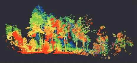
We divided BLS data continuously into circa 10 seconds time patches (Figure 2). The time period was decided according to following reasoning. At first, we took account of forthcoming iterative closest point (ICP) registration, which requires the varying topography of the surface in order to be able to find the correct registration. On this basis, it was visually confirmed that the 10 second period of data typically included sufficient amount of topographic variations. On the other hand, BLS data can include quite fast orientation changes. Therefore, too long time interval would cause patches to include a large variation of slightly different orientations.
Figure 2. An example of a BLS patch. The colour coding spanning from red to blue illustrates the point time within the 10 seconds time patch.
All patches were pre-processed similarly before ICP registration. The AhkhaR2 BLS system creates significant amount of outliers, which were filtered with a voxel-based outlier filtering algorithm (Rönnholm et al., 2015). The next phase was to extract ground points from the point clouds. For this LasTools ground classification algorithm was applied. However, LasTools is designed for airborne laser scanning data, in which case we usually have a full cover of ground points available beneath the canopy. In the case of BLS patches, ground data includes gaps because of occlusions. Therefore, many vegetation points were classified as ground (Figure 3). The remaining non-ground points were manually removed. Ground points of UAV data were classified with LasTools without problems.
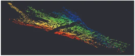
Finally, BLS data was decimated, because the point density close to the scanner is unnecessarily high. For this a 0.10 m grid was created. From each grid element, only the lowest point was selected. An example of a decimated BLS ground point patch is illustrated in Figure 4.
Figure 3. The LasTools classification of ground points (red points) resulted in some misclassified points belonging to the vegetation.
Figure 4. Decimated ground points from a patch. The backpack occludes downwards scanning which can be seen as a linear gap in the middle of the patch.
ICP registration requires an initial registration in order to find the correct registration instead of some incorrect local match. In our case, it appeared that GNSS and IMU information provided sufficient initial registration and no further pre-registration was needed. To minimize the risk of radically false registrations we selected only those UAV laser points that were close to BLS data. For this we created a 0.5 meters grid, which was filled with ones and zeros depending on whether there were any hits from BLS data or not, respectively. This grid assisted in the selection of UAV laser points. All UAV points that were located within the grid cells associated with the number one were selected. UAV data was decimated by utilizing the same procedure as was applied to BLS data. In order to get as much data processing as possible in the same environment, we selected MATLAB’s ICP algorithm for finding registrations. We set UAV data as fixed data and allowed BLS data to move. To ensure numerical stability, ICP requires input data to be quite close to the origin. Therefore, we selected a common origin close to the test area for all the registrations. In addition, point clouds coordinates were temporarily divided by 1000. As a result we got transformation matrices describing the registration translation vector. Because we intended to later correct rotations, Euler angles (φ, θ, ψ) were extracted from the rotation matrices.
In order to visually confirm the ICP registrations, we transformed point cloud patches separately to the common coordinate system (Equation 2). Original points X and transformed points X' are expressed in homogeneous coordinates.
X T
X'= (2)
However, the resulting point cloud does not have much other practical use than a patch-wise visual verification of registrations, because it creates discontinuities between the patches. Therefore, this step is not included in the final workflow (Figure 5).
In order to avoid discontinuities between patches, we applied a linear time-dependent transformation between the centre points of the sequential patches. We modified the original transformation matrix (Equation 1) as a time-dependent transformation matrix
T(t;ϕ+dϕ,θ+dθ,ψ+dψ,TX+dTX,TY +dTY,TZ +dTZ) (3)
In Equation 3 time-dependent corrections to rotations (dφ, dθ, dψ) and shifts along coordinate axes (TX, TY, TZ) are computed
The time difference dt is the distance between the acquisition time of current laser point and the acquisition time of the centre point of the BLS patch. Unit corrections (dφunit, dθunit, dψunit,
dXunit, dYunit, dZunit) were calculated from the orientation
differences between adjacent patches divided by the time difference
Index i identifies the current patch. Notice that the correction in Equation 5 can be applied only to the points in file that has smaller time stamp than the middle point. The points after the middle point need the unit corrections from the next patch. In Equation 5, Δt is the time difference between the centre points of sequential patches.
The final transformation is
In which (X, Y, Z) is an original point, (X’ Y’, Z’) is the transformed point and c is the scale factor of homogeneous coordinates. The rotation matrix Rd is calculated from the
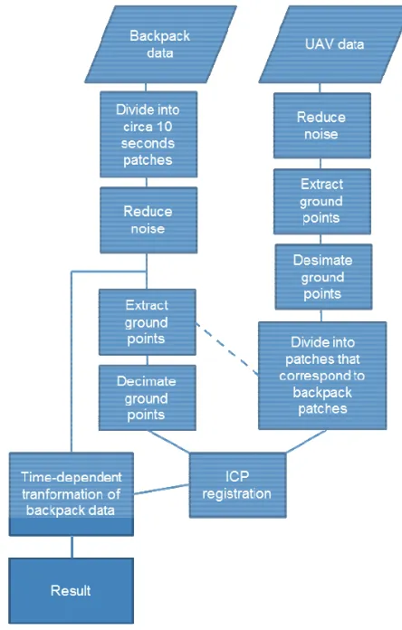
corrected Euler angles (φ +dφ, θ+ dθ, ψ+dψ). The complete workflow of the algorithm is illustrated in Figure 5.
Figure 5. The workflow of BLS registration and correction algorithm.
4. RESULTS
Decimated ground point clouds from BLS and UAV data were registered in 97 patches. The registrations revealed initial average errors of 0.227, 0.073 and -0.083 meters in the easting, northing and elevation directions, respectively. These shifts were estimated for the centre points of the patches. Averages, positive maximums, negative maximums and standard deviations are presented in Table 1.
Easting shift (m)
Northing shift (m)
Elevation shift (m) Positive
maximum 0.803 0.414 0.541
Negative
maximum -0.031 -0.295 -0.670
Average 0.227 0.073 -0.083
RMS 0.274 0.157 0.243
STD 0.174 0.144 0.238
Table 1. The statistics of the initial BLS misalignment.
Even if the average misalignment is relatively small, Figures 6 to 8 reveal that trajectory errors in all directions vary significantly. The misalignment tends to grow first towards some direction, but then after a while to become smaller again. The strong variation of misalignments, however, indicates that the data set has internal orientation errors.
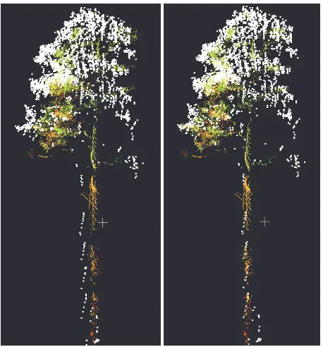
As mentioned in the previous chapter, we also corrected patches with the non-time-dependent transformation. We checked visually the correctness of registrations by opening the transformed BLS points and the original UAV point clouds in the same workspace. Figure 9 presents an example how a clearly visible misalignment in the original BLS data has vanished after the correction.
Figure 6. The misalignment of the BLS patch centre points in the easting direction.
Figure 7. The misalignment of the BLS patch centre points in the northing direction.
Figure 8. The misalignment of the BLS patch centre points in the elevation direction.
In overall, the visual examination revealed that there was no obvious misalignment remaining that could be manually corrected. However, in some patches it was noticed that there were clearly detectable internal mialignments (Figure 10). Still, the alignment usually seemed to match close to one of the alternatives. The example in Figure 10, representing one tree trunk, was the worst case that we could find with the visual examination. We measured interactively the amounts of found internal misalignments. Usually we detected only misalignments smaller than 0.15 m, but in the worst case the shift between the furthest features was aproximately 0.30 m.
Figure 9. The significant planimetric misalignment (left image) was absent after registration and transformation (right image). UAV data is in white colour whereas other colours belong to BLS data.
Figure 10. The sideview (left image) and the topview (right image) of a tree trunk from the time-based corrected BLS point cloud. All visualized data belongs to one patch. As an example, the time difference between blue and green color is circa 3 seconds and between blue and red circa 6 seconds.
Time-based corrections were made to both the full BLS laser scanning data and to the BLS ground point data. For the ground data we applied again the ICP registration process with the original UAV ground data, but we shifted patches with five seconds. The results are illustrated in Table 2 and in Figures 11 to 13. As a result, we observed the average misalignments of 0.084, 0.020 and -0.005 meters for the easting, northing and elevation directions, respectively. The correction of data led to much smaller misalignments than before – as expected. Also, examination of Figures 11 to 13 reveals that misalignments are not variating as much as before. In addition, interactive examination revealed that the largest misalignments can be found in patches that have internal misalignment problems similar to those visible in Figure 10. Figure 14 presents an example, in which the alignment is very good after the time-based correction.
Easting shift (m)
Northing shift (m)
Elevation shift (m) Positive
maximum 0.316 0.261 0.054
Negative
maximum -0.082 -0.144 -0.119
Average 0.084 0.020 -0.005
RSM 0.111 0.058 0.026
STD 0.073 0.055 0.026
Table 2. The statistics of the misalignments after the time-based correction.
Figure 11. The misalignment of the BLS patch centre points in the easting direction after the time-based correction.
Figure 12. The misalignment of the BLS patch centre points in the northing direction after the time-based correction.
Figure 13. The misalignment of the BLS patch centre points in the elevation direction after the time-based correction.
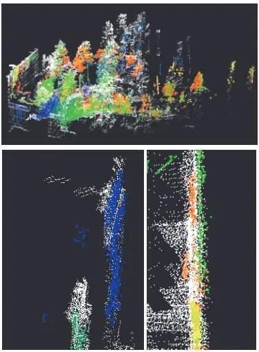
Figure 14. Upper image: An overview of the final resuts after the registration and the time-based transformation. Lower row: two details how BLS laser points (colorful points) are aligned with UAV data (white points) at the wall structures.
5. DISCUSSION
Direct georeferencing sensors have usually difficulties in the forest environment. This was confirmed also in our investigation. The first 20 seconds of the data collection were from a relatively open area. After that the data collection path went in the forest causing significant misalignment as can be seen in Figures 6 to 8. Low satellite visibility and multipath reflections cause inaccuracies to the GNSS observations. In addition, rugged terrain and abrupt turns during the laser scanning together with the rotation drifts of the inertial device cause constantly changing orientation. In Chen et al. (2015) absolute positioning accuracy of combined GNSS and IMU in a typical boreal forest test site was 0.6 m and, interestingly, the maximum misalignments in our test were quite close to that.
The second ICP registration with the corrected BLS data revealed that the result was not ideal. The maximum
misalignment was circa 0.30 m and in many cases the error was over 0.10 m (Figures 11 to 13). One possible reason for this is the presence of internal orientation changes within the patches, which most probably affect negatively to the registration. The cause of that effect warrants a further study. The best candidate for the cause is the smoothing of the forward and reverse solutions used in the GNSS-IMU post-processing for combined trajectory output. Figure 10 reveals that in such case there is no unique solution for the correct registration. Depending on the initial values, ICP registration can fix its solution to a different local minimum when there is no exact match available. Another disadvantage of ICP is that it requires enough variation in terrain to function properly. Usually, a natural terrain patch is not flat, but this can become an issue when terrain is close to a plane and data is blurred because of internal orientation changes, for example.
It is clear that our linear time-dependent correction model could not describe all the internal changes of orientations within the BLS patches. Therefore, the initial assumption of the steady behaviour of orientations proved to be wrong. The combination of abruptly changing orientation and the serpentine trajectory of data acquisition distribute data unevenly between the sequential patch centres. Because our method was data-driven, no trajectory information was utilized leaving details of data acquisition path unknown.
In the future, the sensor-driven model should be examined, in which scanning trajectory and raw observations are taken into account. Another future research subject is to improve the automatic classification of ground points. The small size of BLS data patches is especially challenging because measured terrain points can be fragmented, under some vegetation there are no ground points available, and obstacles may cut the lower parts of vegetation very sharply making such areas appear identical to a terrain slope. The current ground point classification methods are not optimal for our case. Even if this part made our algorithm semi-automatic, there is a high potential to make the whole process fully automatic.
We selected UAV data as the reference. UAV orientations rely also on GNSS and IMU devices, and the RMSE of ground points is typically reported to be 0.08-0.09 meters (Jaakkola et al., 2010; Flener et al. 2013; Tulldahl et al., 2015). However, the advantage of UAV data collection is that typically there are no obstacles blocking the satellite visibility. Therefore, orientations are usually not changing as rapidly than with BLS data acquired in the forest environment. In other words, even if UAV data may include inaccuracies it is significantly more accurate than BLS data collected in forests and therefore suitable as the reference. In addition, collecting the reference with any other method would require much more effort. If available, however, UAV data could be replaced by, e.g., TLS data, or even high density ALS.
6. CONCLUSIONS
Our goal was to evaluate the quality of BLS data. For this purpose, we developed a novel process in which BLS data was compared with UAV data in small patches. Data processing included noise filtering, division of data into patches, ground point extraction, data decimation, and ICP registration. As a result, we managed to see the behaviour of data from circa 10 seconds intervals. Our evaluation revealed initial average misalignments of 0.227 m, 0.073 and -0.083 in the easting,
northing and elevation directions, respectively. Even if the averages were reasonably small, the maximum misalignments were as large as 0.803, 0.414 and -0.670 meters revealing a need for correction. Because these results are relative to UAV observations that create a point cloud of 0.08-0.09 meters RMSE accuracy, absolute misalignments may have additional variation of this magnitude.
We applied a time-based linear correction to BLS data according to the results of the ICP registration to UAV data. The time-based approach ensured that data remained continuous after the correction. The corrections were defined using the sequential orientation differences of patches. After the correction of the BLS data, ICP registration was run again. The correction of data resulted to average misalignments of 0.084, 0.020 and -0.005 meters in the easting, northing and elevation directions, respectively. The interactive examination verified that in most cases registration and time-based BLS data correction were successful. Also, the maximum misalignments, 0.316, 0.261 and -0.119 meters, were smaller than before the correction. The possible reasons for these maximum misalignments were the short-term internal variation of orientations within the patches and possibly too little variation in the terrain shape. The linear correction model could not compensate all the misalignments. To overcome this problem, further research on applying a better correction model is needed.
ACKNOWLEDGEMENTS
The authors would like to thank Academy of Finland for financial support through projects “Centre of Excellence in Laser Scanning Research (No. 272195)”, Strategic Research Council project COMBAT (No. 293389) and “Interaction of Lidar/radar beams with Forests using mini-UAV and mobile forest tomography”. The research leading to these results has received funding from the European Community's Seventh Framework Programme ([FP7/2007-2013]) under grant agreement n° 606971.
REFERENCES
Chen, G., Kua, J., Shum, S., Naikal, N., Carlberg, M., Zakhor, A., 2010. Indoor Localization Algorithms for a Human-Operated Backpack System. In Proceedings of the 3D Data Processing, Visualization, and Transmission, Paris, France, 17– 20 May 2010, 8 pages.
Chen, Y., Tang, J., Kaartinen, H., Karjalainen, M., Hyyppä, J., 2015. Accuracy of MLS positioning inside the forest using IMU GPS and SLAM. Report of Advanced Techniques for Forest Biomass and Biomass Change Mapping Using Novel Combination of Active Remote Sensing Sensors Collaborative project, 23 pages.
El-Sheimy, N.,2005. An Overview of Mobile Mapping Systems. In Proceedings of FIG Working Week 2005 and GSDI-8, Cairo, Egypt, 16–21 April, 24 pages.
Ellum, C. and El-sheimy, N., 2000. The development of a backpack mobile mapping system. International Archives of the Photogrammetry, Remote Sensing and Spatial Information Sciences, 33, pp. 184–191.
Elseber, J., Borrman, D., Nüchter, A., 2013. A study of scan patterns for mobile mapping. International Archives of the Photogrammetry, Remote Sensing and Spatial Information Sciences, 40(7/W2), pp. 75–80.
Glennie, C., Brooks, B., Ericksen, T., Hauser, D., Hudnut, K., Foster, J., Avery, J., 2013. Compact Multipurpose Mobile Laser Scanning System — Initial Tests and Results. Remote Sensing, 5(2), pp. 521–538. doi:10.3390/rs5020521
Flener, C., Vaaja, M., Jaakkola, A., Krooks, A., Kaartinen, H., Kukko, A., Kasvi, E., Hyyppä, H., Hyyppä, J., Alho, P., 2013. Seamless Mapping of River Channels at High Resolution Using Mobile LiDAR and UAV-Photography. Remote Sensing, 5(12), pp. 6382-6407. doi:10.3390/rs5126382
Jaakkola, A., Hyyppä, J., Kukko, A., Yu, X., Kaartinen, H., Lehtomäki, M., Lin, Y., 2010. A Low-Cost Multi-Sensoral Mobile Mapping System and Its Feasibility for Tree Measurements. ISPRS Journal of Photogrammetry and Remote Sensing. 65, pp. 514–522.
Kukko, A, Kaartinen, H., Hyyppä J., and Chen, Y., 2012. Multiplatform Mobile Laser Scanning: Usability and Performance. Sensors, 12(9), pp. 11712–11733.
Kukko, A., Kaartinen, H. Zanetti, M., 2015. Backpack Personal Laser Scanning System for Grain-Scale Topographic Mapping. 46th Lunar and Planetary Science Conference, The Woodlands, TX, USA, Abstract #2407, 2 pages.
Lauterbach, H., Borrmann, D., Hess, R., Eck, D., Schilling, K., Nüchter, A., 2015. Evaluation of a Backpack-Mounted 3D Mobile Scanning System. Remote Sensing, 7(10), pp. 13753– 13781. doi:10.3390/rs71013753
Leica. http://www.leica-geosystems.com (accessed 23.11.2015).
Liang, X., Kukko, A., Kaartinen, H., Hyyppä, J., Yu, X., Jaakkola, A., Wang, Y., 2014. Possibilities of a Personal Laser Scanning System for Forest Mapping and Ecosystem Services. Sensors, 14(1), pp. 1228–1248. doi:10.3390/s140101228
Naikal, N., Kua, J., Chen, G., Zakhor, A., 2009. Image Augmented Laser Scan Matching for Indoor Dead Reckoning. Proc. of the IEEE/RSJ International Conference on Intelligent Robots and Systems (IROS), pp. 4134–4141.
Nüchter, A., Borrmann, D., Koch, P., Kühn, M., May, S., 2015. A man-portable, IMU-free mobile mapping system. ISPRS Annals of the Photogrammetry, Remote Sensing and Spatial Information Sciences, 2(3/W5), pp. 17–23.
Owari, T., Kasahara, H., Oikawa, N., Fukuoka, S., 2009. Seasonal variation of global positioning system (GPS) accuracy within the Tokyo University Forest in Hokkaido. Bulletin of the Tokyo University Forests, 120, pp. 19–28.
Rönnholm, P., Kukko, A., Liang, X., Hyyppä, J., 2015. Filtering the outliers from backpack mobile laser scanning data. The photogrammetric journal of Finland, 24(2), pp. 20–34. doi: 10.17690/015242.2
Tulldahl, M., Bissmarck,, F., Larsson, H., Grönwall, C., Tolt, G. 2015. Accuracy evaluation of 3D lidar data from small UAV. Proc. of SPIE Vol. 9649, 11 pages.