MODELLING THE CONSTRAINTS OF SPATIAL ENVIRONMENT IN FAUNA
MOVEMENT SIMULATIONS: COMPARISON OF A BOUNDARIES ACCURATE
FUNCTION AND A COST FUNCTION.
L. Jolivet a, *, M. Cohen b, A. Ruas caCOGIT, Institut national de l’information géographique et forestiè
re, 94160 St-Mandé, France – [email protected] b
Université Paris Sorbonne, UMR ENeC, 75000 Paris, France – [email protected] c
Laboratoire COSYS-LISIS, IFSTTAR, F-77447 Marne-la-Vallée, France - [email protected]
Commission II, WG II/4
KEY WORDS: Modelling, Simulation, Geographical databases, Landscape, Fauna, Movement, Experimentation, Indexes
ABSTRACT:
Landscape influences fauna movement at different levels, from habitat selection to choices of movements’ direction. Our goal is to provide a development frame in order to test simulation functions for animal’s movement. We describe our approach for such simulations and we compare two types of functions to calculate trajectories. To do so, we first modelled the role of landscape elements to differentiate between elements that facilitate movements and the ones being hindrances. Different influences are identified depending on landscape elements and on animal species. Knowledge were gathered from ecologists, literature and observation datasets. Second, we analysed the description of animal movement recorded with GPS at fine scale, corresponding to high temporal frequency and good location accuracy. Analysing this type of data provides information on the relation between landscape features and movements. We implemented an agent-based simulation approach to calculate potential trajectories constrained by the spatial environment and individual’s behaviour. We tested two functions that consider space differently: one function takes into account the geometry and the types of landscape elements and one cost function sums up the spatial surroundings of an individual. Results highlight the fact that the cost function exaggerates the distances travelled by an individual and simplifies movement patterns. The geometry accurate function represents a good bottom-up approach for discovering interesting areas or obstacles for movements.
* Corresponding author
1. INTRODUCTION
1.1 General context
The context of our research refers to landscape planning. When defining projects, planners need to have knowledge and insight on ecosystem functioning. Animal species represent parts of current ecosystems. We focus on how fauna movement can be taken into account within future projects. Movements play a part in the survival of individuals and act upon the environment. Movement patterns depend on the species as they have different needs and ability to move. Patterns are also related to the general type of environment where a species lives and at a more precise level to the characteristic of its home range.
An important aspect to recall is that knowledge on animal species requires a great amount of field work framed by precise protocols. Electronic devices such as radio and satellite-based technologies help to increase the amount of information on where individuals go and how they move. Spatial features are described in databases created from field work and from remote sensing techniques. Databases tend to be enriched and more accurate, in particular concerning attributes and spatial unit aggregation on land cover and land use. The selection of the data needed for a particular analysis is a problematic tackled by Geographical Information Science. The problematic includes being able to define what is the quality of the data and how it propagates in the results (Devillers et al., 2007). It also includes at what scale data should be considered (Wilkin et al., 2007)
and how they should be analyzed and the results interpreted (Li & Wu, 2004). Factors such as the trophic specialization rank of species can be taken into account while defining what spatial features should be studied. The more specialized species are, the more dependent to its environment they tend to be (Holt, 1996). Besides, perception of environment depends strongly on the species (Tolman, 1948; Von Uexküll, 1934).
Field information and recordings contribute to the knowledge on animals. Though, it cannot be exhaustive as all study sites and species cannot be scanned and followed. In parallel, the need in landscape planning is to visualize effects of future project on movements. Modelling allows formalizing concepts and mechanisms at stake in the movement patterns of an individual. Then it allows testing scenarios corresponding to projects. Virtually modifying a landscape enables to observe consequences by comparing simulated movements before and after modification. In this article, the initial need was to be able to simulate movements in order to test the expected effects of planning projects.
1.2 Previous works and our problematic
Modelling fauna movement implies identifying what acts upon it. Elements influencing fauna movement are from different sources. They come from the environment: living environment (other individuals, microorganisms including bacteria for instance), spatial surroundings (e.g. landscape features, minerals flux and pollution particles), other variables like acoustic and
light. Another aspect to be taken into account lies in the characteristics related to the species. These characteristics depend on the animal species, its capacity and needs for living. The landscape elements will not have the same effect depending on the species. Habitat preferences are defined partly by the geophysical features like relief (Dickson & Beier, 2007) and by components like vegetation type and cover (Bélisle et al., 2001). To define models on animal movements, it is necessary to identify hindrances and corridors. These two functions are linked to certain habitat (where animal lives) and travel areas (where they move) preferences. Preferred places can be located and characterised by comparing the proximity of individuals during their usual activities and larger surroundings (Matthiopoulos, 2003).
A large number of models for animal movements have been defined. General models can be listed in several categories including: cost functions, object-oriented, statistical. Approaches relying on cost functions generally divide studied areas in regular units. For each unit, landscape elements are associated with a cost value and a function estimates the cost, or the facility, for individuals to move from a starting point towards various directions (La Morgia et al., 2011; Palmer et al., 2011). Object-oriented programming formalizes explicitly the characteristics and the properties of individuals as well as those of their environment (Vuilleumier & Metzger, 2006). What we called statistical approaches integrates equations that evaluate the probability of movement in a direction. It can use for instance on differential equations such as in Coulon et al. (2008). Modelling movements can rely on random walks like in Miller & Maude (2010). The parameters of the different approaches have to be fixed depending on the objectives of the study. Various types of movements (daily, seasonal migrations, dispersal) can be modelled by changing the values of the parameters, as well as the studied influence on movement patterns (landscape, other individuals) can be.
Our work stands in the modelling of movement within a geographical space. It focuses on the characterization of this space depending on the species. Our contribution is to use high-scaled data describing spatial environment, these data being available for the whole French territory. From these data, we aimed at formalizing the influence of each type of landscape features depending on study cases. We worked on medium-sized animal species which movements are coherent with the databases used to describe space. Some problematics are related to data quality. Qualification of data is a major issue in analyzing processes and in re-exploiting the data for assessment objectives. From the fauna movement analysis, it can be noticed that the data used for discovering and corroborating knowledge are central. Indeed several aspects in data intervene, in particular:
– Geometrical accuracy – Exhaustiveness of the cover – Attribute definition and details
Spatial scale is defined depending on the adaptability of data to the represented element or phenomenon. It depends on geometry accuracy and spatial aggregation. Temporal accuracy is linked to the time separating updates and the adequacy between the date of the data and the reality at that moment. Our problematic is to define what are the data needed for understanding and representing fauna movements and how these data can be treated to be used in evaluating landscape planning projects. This question is tackled from a movement simulation proposal.
2. OBJECTIVE AND PROPOSAL OF MOVEMENT-SIMULATION MODEL
2.1 Objective and approach
Our main objective is to propose a simulation model for movements. Modelling fauna movement is quite a challenge as many parameters are involved. This is why we focused on the interactions between animal species and landscape features. We also have limited the scope to daily movement. We aimed at defining a model that formalizes a) the influence of landscape features on movements, b) for more realism, movement patterns in terms of travelled distances and activity rhythms. We implemented the model in order to be able to simulate trajectories. Then changing the spatial environment will allow to visualise the consequences of modifications on the simulated trajectories and so to formulate hypotheses about the possible consequences on real fauna movements. We believe that modelling all the elements that influence and define the patterns of animal movements would be too complex. Being aware of that complexity, we have chosen to focus on only one part of the influence and to exploit existing data for sake of clarity. The application of such modelling is more in landscape planning, including communication towards stakeholders and base for debates, than in trying to discover new animal behaviours.
Our global approach first consisted in gathering information on animal movements depending on the species. Then we proposed a model that formalizes available data and knowledge on individuals’ behaviours and the relations between individuals and their environment (part 2). We present in the next section our proposed model. We detail the approach for simulating trajectories which is based on agent-oriented modelling. In the results (part 3), we focus on the last part of the global methodology: two simulation functions that have been proposed and tested.
2.2 Material and methods
2.2.1 Data and knowledge for modelling: To establish a
model, we needed to have knowledge about the influence of landscape on animals. Three types of sources were exploited: literature, experts and data analyses. We analysed particular study cases with their corresponding datasets. Then we faced the results with previous conclusions on works described in literature, especially literature in ecology for the spatial behaviours and apprehension of landscape elements depending on the species.
The databases on animal movements we had access to, contain GPS tracking recording from collars. Several species were concerned. Though, in this article, we only focus on the study case of red foxes in an urbanised environment. Data come from an existing survey led by the ANSES agency. The GPS recordings have an average time interval of 15 minutes during 24 h for 4 individuals. In this dataset, it is considered that the GPS planimetric coordinates were accurate within about 20 m. The urban environment contains masks for satellite signal such as buildings. Wooded vegetation has likewise a masking effect that can happen when foxes stay in patches to rest or to hide. We did not use the coordinates Z given by the GPS as the accuracy can be less than within 20 m. We have chosen to use the projection on the DTM. The data describing the spatial environment are from diverse institutional sources. BD TOPO® and DTM from RGE®ALTI are produced by the French mapping agency IGN. BD TOPO® is a metric database, meaning that the objects are digitized within 1 meter accuracy.
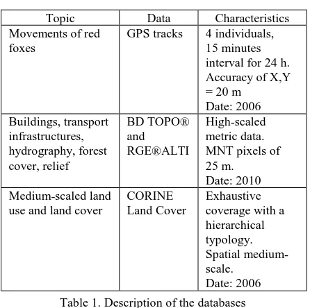
It includes more than 95 % of the buildings and more than 98 % of road network. Main forest stands are indicated. Nevertheless, some themes are excluded like crop fields. The European database CORINE Land Cover takes into account homogenous land cover larger than 0.25 km². It is generally used for medium-scale mapping. The advantage of this database is that it characterizes the land cover continuously thanks to a typology. Characteristics of the databases are given in Table 1.
Topic Data Characteristics
Movements of red foxes
GPS tracks 4 individuals, 15 minutes interval for 24 h. Accuracy of X,Y = 20 m
Date: 2006 Buildings, transport
infrastructures, hydrography, forest cover, relief
BD TOPO® and RGE®ALTI
High-scaled metric data. MNT pixels of 25 m. Date: 2010 Medium-scaled land
use and land cover
CORINE Land Cover
Exhaustive coverage with a hierarchical typology. Spatial medium-scale.
Date: 2006
Table 1. Description of the databases
A first step was to analyse the data. We have based the analyses on the comparison between landscape elements near the individual and the ones further. This allows the extraction of preferred landscape elements and the ones that are avoided or that can hinder movements. We don’t present those analyses in this article (details can be found in Authors-xx). The accuracy of the input data impacts on the detected spatial behaviours. Spatial preferences for particular land covers could be identified, as well as avoidance to transport infrastructures. Though the exact place where an individual crosses a road or the pattern of his movement to by-pass buildings are unknown. It is not only a matter of completeness and accuracy in the data describing the study site but also a matter of capacity of the tracking devices. Results from the analyses of the study cases were then confronted to the literature. Our aim was not to discover new behaviour but to characterize properly the movement in our study cases. This would enable the construction of the concepts relevant in our model. The model focuses on the type of influence associated with the landscape features. We present the identified influences in the case of the red fox in the next section (2.2.2). These correspond to the conceptual knowledge as input in the model. Four types of roles for landscape features were determined:
- Obstacle
- Corridor for movement - Interesting element - Avoided element
The influences associated to landscape features depend on the animal species. For red fox, the knowledge we defined in the model is synthetized in Figure 1.
Figure 1. Knowledge on red fox movements in peri-urban environment and the influence of landscape features.
Red fox is a generalist species that can adapt in various environments. We focused on the case of peri-urban area. Individuals were observed covering large distances at night, until 10 km, included in an area of around 1.5 km². The given values are an average for the four individuals. Landscape features are linked to diverse roles. For example, railway lines can reduce crossings, though their surroundings can be corridors due to the vegetation and to low human disturbance.
2.2.2 The agent-based simulation model: Our proposal for
simulating movements is agent oriented. An agent is an individual. The environment includes landscape features with geometry and attributes on their characteristics and their influences. Activities are indirectly enclosed in the two phases: a phase during daytime corresponding to small movements and a phase for nocturnal foraging. In the model, we favoured the second phase corresponding to larger movements as well as the relations between individuals and landscape features. As a consequence, the results are simulated trajectories on longer distances than the ones usually travelled by an individual for 24 h. We are interested on daily movements. Thus we left aside the dispersal and migration dynamics.
The strategy for construction a trajectory is as follow:
(1) The agent records its location and perceives its spatial environment within a radius.
(2) The agent selects an element as a destination. This element is chosen if it is inside the perception radius and if it corresponds to the more accessible (less obstacles in between) and to the largest interesting area (building or vegetation patch as described in Figure 1 – commercial and industrial areas are not considered here are they correspond to typology classes).
(3) The agent moves towards the destination step by step. It calculates its trajectory thanks to one of the two functions that we will evaluate and to a medium speed.
(4) When the agent reaches the destination, it stays included (vegetation patch) or around (building) such if it exploits the potential resources.
We developed two functions for the calculation of constructing the trajectories. The first function takes into account the boundaries of the landscape elements. The second function relies on cost valuation of how elements hinder or facilitate movements. The model on knowledge presented in Figure 1 remains valid for the two methods. Figure 2 illustrates the principle of the two functions.
I = Σ I_favour + Σ I_obstacle + Σ I_direction
Figure 2. Overview of the principle of the two functions for an agent to build a trajectory between its actual location and the selected destination: 1) the first function takes into account the
geometry of landscape features; 2) the second function calculates a cost value for movement.
We present the results in section 3, the details of the functions with the protocol implemented for evaluating their advantages and drawbacks.
3. RESULTS
We first present the results of animal movements depending on the trajectory simulation functions, and then, we analyse the results.
3.1 The proposed two trajectory functions
We have proposed two simulation functions in order for an agent to be able to build its trajectory. Our concern focuses on step (3) of the strategy for simulation: a destination has been selected and the agent is heading towards it. The two methods differ about the consideration of spatial environment. The roles of landscape elements depend on the species, here the red fox.
3.1.1 Function (a), boundaries accurate: The first method
takes into account the boundaries of the features as shown in Figure 3. This statement implies that obstacles are avoided. Buildings are walked around. A permeability value has been attributed to roads, railways and water lines according to their importance (traffic intensity and width). The vegetation patches are destinations as they represent interesting elements especially for hiding.
Figure 3. The object-accurate function: the points of the trajectory built step by step by an agent. In this example, buildings are avoided and roads have permeability values.
3.1.2 Function (b), interest sum: The second method
summarizes the cost values of the landscape elements around an agent. The spatial environment around the agent is considered inside a circle divided in sections. The direction taken by the agent is in the direction of the section with the lower cost and so with the higher value given by our interest function. The interest function is defined as follow (1).
(1)
where I = total interest for movement associated to a section I_favour = index for the presence of corridors in the section (vegetation)
I_obstacle = index depending on the number of obstacles (buildings, roads, railways, waterlines)
I_direction = index for the direction of the section All indexes used in the sums in function (1) are whole number between 0 (high-cost section for movement) and 3 (low-cost section). The function is illustrated in Figure 4.
Figure 4. The interest function: it takes into account the cost value of landscape elements for movement. In that example, half a circle represents the surroundings of the agent. It is divided in 5 equal sections and its main direction is towards the destination. The more interesting the section is, the redder it is.
3.2 Experiments on the two trajectory functions
3.2.1 The defined protocol: Our protocol to evaluate
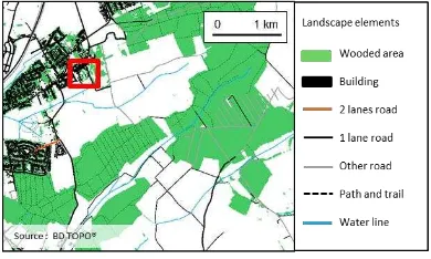
differences between the two proposed simulation functions is to launch 50 trajectories in the same initial conditions for each trajectory function. The whole simulation strategy has a random part, when an agent selects destinations step by step. The study site is located in the suburb area of Nancy in the East of France, shown in Figure 5. This site is mainly covered by forests. Grassland and agricultural fields are not present in the dataset (represented by white background on the map in Figure 5). On the west part of the site, a town centre and a residential area is located.
Figure 5. The study site in the east of France covers 15 km². It is mainly forested with urbanised area on the west part. The red
rectangle corresponds to the area shown in Figure 6.
Some parameters have to be defined. The parameters are divided between those identical for the two functions and those that differ due to their specific inputs. We present the values in Table 2.
Table 2. Values of the parameters
The values of the parameters were settled based on hypotheses on the environment perception ensued from the knowledge corpus. We have run tests in order to evaluate the effects of parameters values on the results and to determine which was the more likely close to reality. The medium speed is the average of the estimated speeds between GPS points during 24 h. The model integrates a decrease of the speed when an obstacle is encountered. We fixed the general perception radius of the spatial environment at 200 m. This value is a hypothesis as there is no unique value for such perception depending on the type of environment at a certain time of the individual. We ran some simulation tests with different values from 10 m to 500 m. The more coherent results in terms of covered surfaces correspond to the values between 50 m and 200 m. We took the higher value to fit with the high-scaled function (boundary accurate) and the medium-scaled one (interest sum). In the interest sum function, the sections are defined to be a compromise between calculation time and the accuracy of the consideration of spatial environment. For instance, if the number of sections is increased, the cut-out of space might end up with areas that would be too small to differ from their neighbours. The distance of 50 m has been fixed in order to be smaller than the perception radius and to be coherent with the distances covered between the simulated points. The possible re-selection of destinations is set for the red fox species as it has been observed from the GPS data. Probabilities of crossing obstacles were set in order to fit with global knowledge on the permeability of the diverse linear landscape elements. There are no values that can fit every elements and also context of crossings (e.g. necessity, exploration). It is also an objective of the model to allow modifying values of parameters to test and
3.2.2 Simulated trajectories obtained with the two functions: We launched the two simulation functions for the
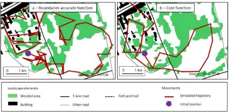
boundary accurate function and the cost function. This allows to map and to explicitly compare the results of the two functions. The experiments were run for a time length of 24 h for agent standing for red fox individuals. Time length between simulated points is 2 minutes. A visual comparison is given in Figure 6. The initial point is located at the south border of an urbanised area and the majority of trajectories are located in and around this town.
Figure 6. Two trajectories constructed with the two simulation functions, extraction concerning one hour. We notice that the
one built from the boundaries accurate function (a) is more sinuous than the one build with the cost function (b).
We defined criteria to compare quantitatively the two functions. Criteria deal with the form of the trajectory and with the relations between a trajectory and landscape elements. Table 3 gives the average concerning the 50 trajectories for several criteria.
Table 3. Comparison of the two functions based on criteria, calculated for a 24 h simulation. Calculations are made from the
simulated locations, related to geographical objects. The main difference lies in the total distance.
The first remark on the calculated criteria is that distance from the cost function is longer than from the boundaries accurate one. First, both functions largely exaggerate the distances as the model insists on representing movements. Besides, we did not integrate the difference between day and night. Second, the difference between the two functions comes from the fact that the cost function is less sinuous than the other function. Indeed, paths are chosen depending on the direction assigned with the less cost. There is no bypassing around buildings or when a road has to be crossed. When the agent exploits the reached destination, it stays inside or near the destination (phase 4 in the strategy in 2.2.2). In both functions, we fixed the time length of the exploitation at 10 minutes. It is quite short. For a 2 minutes time length, it corresponds to 5 simulated points. This contributes to the increase of the covered distances as the agent is in fact still moving during the exploitation, even if the
distance can be shorter in case of obstacle with the reduction of the speed.
The relations between simulated trajectories and wooded areas are quite similar in the two functions such as the medium distance to roads (all types: with low and strong traffic). Though, the majority of roads are associated with medium traffic and for this type of roads, the cost functions is associated with larger average distance. This is partially due to the fact that trajectories from cost function can be located in areas far from the urbanized area, so as a consequence far from roads. This last point is also the explanation to the difference in numbers of different wooded areas crossed, as cost function corresponds to larger distances.
3.3 Discussion
The process of modelling always introduces a simplification of reality. In fauna movements, the complexity of the influencing factors led us to focus on landscape elements available in existing produced geographical databases. We aimed at selecting few aspects of the animal behaviours in the simulation process so that to be able to interpret the simulation results and to be able to adapt it. The comparison of two spatial information considerations allows identifying the relevancy of each consideration in fauna movement simulations. From the results of simulated trajectories based on the study case of red foxes, we stated that the two functions are adapted to a certain spatial and temporal scale. The function that integrates accurate geometries of geographical objects allows a precise modelling of the known influence of geographical features on movements. This function is bottom-up in the discovery of trajectory patterns. The details of the trajectories around and through elements are interesting if they make sense in terms of influence of landscape features. We focused on the global pattern of the trajectory and the spatial preferences and obstacles rather than on the formalisation of the exploitation of precise landscape elements. The second function is based on a cost calculation for effort needed to be generated by the animals. It summarizes in the neighbourhood of an individual the presence and amount of features that would facilitate or hinder movements.
The boundaries accurate function corresponds to high scaled data, whereas the cost function can be qualified as a function describing the spatial environment at medium scaled. Though, this medium scaled view of the spatial environment is made possible thanks to high-scaled databases. The consideration of spatial environment is also linked to temporal aspect and to type of movements. Taking into account the geometry of landscape features is relevant if movements are studied at a fine temporal scale, such as in Coulon A. et al. (2008) and Dickson & Beier (2007). In our datasets of observations, daily movements were described. It was convenient to have high frequency of GPS recordings for locations so that to analyse the more precisely as possible tracks taken by animals as well as the influence of landscape elements on directions. The accuracy of the GPS tracks is quite adequate with the high-scaled spatial data. Despite positioning errors, it allows estimating the global trend of an animal’s locations in relation to the landscape features. Simulations were undertaken with a time length of 2 minutes, which is very high frequency. This simulation frequency is coherent to the representation of bypassing buildings, roads or other obstacles, even if the description of how an individual goes around buildings and other obstacles can only be estimated in the observation datasets. We can say that the boundaries accurate function is more realistic than the cost function. Though, it can be long to calculate (for instance in densely
urbanised areas). Besides it is sometimes difficult to model the exact movement behaviour of an animal that would be relevant at that high level of accuracy. Indeed, observation data, even with high frequency cannot always be precise enough to clearly understand how and where an animal apprehend landscape features (e.g. where and how roads are crossed).
Dispersal movements are generally on larger distances than daily movements, such as single long-distance movements for exploration. The cost function might be more relevant in that type of movement like in La Morgia et al. (2011), even if Vuilleumier & Metzger (2006) uses a vector-based description of space for long-distance movements. In our tests, the simulated trajectories are less sinuous as space units are considered and global direction is decided from the analysis of the units. This can be associated with a lower consideration for the quality of geometrical information. Though, it can be clearer for identifying areas of corridors or obstacles, to not consider
High-scaled geographical data are taken into account Precise apprehension of landscape features
Daily movement and its influence of landscape elements (b) Cost function: case of simulating different types of movements: landscape elements can have various influences or importance during a daily movement inside a home range comparing to a migration.
For the evaluation of the results, the same study area is concerned, same as the site where GPS data have been analysed. We can say that the quality of data analyses depends on the quality of the input data. Concerning the description of land cover types and the one of specific landscape features, the completeness of the themes influences the detection of spatial preferences. Besides, it is necessary to have access to interesting attributes on the spatial elements (e.g. type and structure of vegetation patches). The accuracy of the geometry in the spatial description and in the movements’ data allows misinterpretation of animal behaviour and its spatial preferences. In the data analyses, we have noticed that relevant landscape elements are missing in the dataset used for describing spatial environment. The enrichment depends on the species. For foxes, it can be relevant to have more precise information on favourable resources areas like agricultural fields or urban patches with little disturbance. Other useful data could be about hedgerows that can act like corridors and physical barriers such as fences. We assume that this note is also valid for simulation process. Simulated trajectories could be improved with an enrichment of the environment. In that case, the simulation model could increase the realism of movements with better modelled interactions between individuals and space.
4. CONCLUSIONS
We have presented a model for simulating daily animal movements based on the influence of landscape features. We have developed two functions in order to calculate trajectories. We saw that each function was related to a certain spatial scale of geographical data. Our function taking into account
geometries of buildings is interesting as it is a bottom-up approach for discovering global patterns in simulated trajectories and to link them to the landscape description at fin or regional scale. Summarising the geographical information, as we did with the cost function, decreases quality of the description of spatial environment. It is useful to have a synthetic view of the potential paths along where animals would go. Our agent-oriented approach can accept the addition of some individual parameters like personality parameters for individuals (e.g. boldness, perseverance) and more generally the individual’s characteristics that can greatly influence some types of movements (e.g. migration, exploratory).
The perspective is to test the method on another species. We mentioned that we have worked and analysed data on roe deer as well as on red deer. Their movement patterns are quite different due to their needs. They are herbivores which, among other aspects, lead them to exploit specific landscape elements as resources. It would be interesting to see how the two functions of simulation fit their movements’ rhythms and paths, and which adaptations should be brought. With a well-parametrized model and a relevant consideration of spatial environment, landscape planning projects can be assessed in order to precise the type of concrete action and their best location.
ACKNOWLEDGEMENTS
The authors would like to thank the providers of the GPS data on foxes, especially E. Robardet and the French Agency for Food, Environmental and Occupational Health & Safety (ANSES).
REFERENCES
Bélisle M., Desrochers A., Fortin M. J., 2001, Influence of forest cover on the movements of forest cover on the movements of forest birds: a homing experiment. Ecology, 82(7), pp. 1893-1904
Coulon A., Morellet N., Goulard M., Cargnelutti B., Angibault J.-M., Hewison A. J. M., 2008, Inferring the effects of landscape structure on roe deer (Capreolus capreolus) movements using a step selection function. Landscape Ecology, 23, pp. 603-614
Devillers R., Bédard Y., Jeansoulin R., Moulin B., 2007, Towards spatial data quality information tools for experts assessing the fitness for use of spatial data. International journal of Geographical Information Science, 21(3), pp. 261-282
Dickson B. G., Beier P., 2007, Quantifying the influence of topographic position on cougar (Puma concolor) movement in southern California, USA. Journal of Zoology, 271, pp. 270-277
Holt R. D., 1996, Food webs in space: an island biogeographic perspective. In: Food Webs: Contemporary Perspectives, G. Polis and K. Winemiller (Editors), pp. 313-323
La Morgia V., Malenotti E., Badino G., Bona F., 2011, Where do we go from here? Dispersal simulations shed light on the role of landscape structure in determining animal redistribution after reintroduction. Landscape Ecology, 26, pp. 969-981
Li H., Wu J., 2004, Use and misuse of landscape indices. Landscape Ecology, 19, pp. 389-399
Matthiopoulos, J., 2003, The use of space by animals as a function of accessibility and preference. Ecological Modelling, 159(2-3), pp. 239-268.
Miller J. A., Maude G., 2010, Using correlated random walks to analyze interaction between Brown Hyena pairs in Northern Botswana. In proceedings of GIScience, Zurich, Switzerland (15-17 Sept. 2010)
Palmer S. C. F., Coulon A., Travis J. M. J., 2011, Introducing a “stochastic movement simulator” for estimating habitat connectivity. Methods in Ecology and Evolution, 2(3), pp. 258-268.
Tolman E. C., 1948, Cognitive maps in rats and men. Psychological Review, 55(4), pp. 189-208.
Von Uexküll J., 1934, Mondes animaux et monde humain, followed by Théorie de la signification. Denoël Ediction, 1965, Paris.
Vuilleumier S., Metzger R., 2006, Animal dispersal modelling: Handling landscape features and related animal choices. Ecological Modelling, 190, pp. 159-170
Wilkin T.A., Perrins C.M., Sheldon B.C., 2007, The use if GIS in estimating spatial variation in habitat quality: a case study of lay-date in the Great Tit Parus major. IBIS, 149(2), pp. 110-118