FAST AND ACCURATE VISIBILITY COMPUTATION IN URBAN SCENES
Bruno Vallet and Erwann Houzay
Universit´e Paris Est, IGN, Laboratoire MATIS 4, Av. Pasteur
94165 Saint Mand´e Cedex, FRANCE
bruno.vallet@ign.fr (corresponding author), erwann.houzay@ign.fr http://recherche.ign.fr/labos/matis
Working Groups I/2, III/1, III/4, III/5
KEY WORDS:Photogrammetry, Visibility, Mobile mapping, Building facade, Urban Scene
ABSTRACT:
This paper presents a method to efficiently compute the visibility of a 3D model seen from a series of calibrated georeferenced images. This is required to make methods aimed at enriching 3D models (finer reconstruction, texture mapping) based on such images scalable. The method consists in rasterizing the scene on the GPU from the point of views of the images with a known mapping between colors and scene elements. This pixel based visibility information is then made higher level by defining a set of geometric rules to select which images should be used when focusing on a given scene element. The visibility relation is finally used to build a visibility graph allowing for efficient sequential processing of the whole scene
1 INTRODUCTION
One of the most investigated applications of mobile mapping is the enrichment an existing 3D urban model (obtained from aerial photogrammetry for instance) with data acquired at the street level. In particular, the topics of facade reconstruction (Frueh and Zakhor, 2003) and/or texture mapping (B´enitez et al., 2010) have recently received a strong interest from the photogramme-try and computer vision communities. An important step in such applications is to compute the visibility of the scene, that is to answer to the questions:
• Which scene element is visible at a given pixel of a given
image (pixel level)
• Which scene elements are seen well enough in a given
im-age, i.e. for which scene elements does the image contain significant information (image level)
Depending on the applications, these questions can be asked the other way, that is querying the images/pixels seeing a given scene element or 3D point. In practice, mobile mapping generates a large amount of data, and an acquisition led on an average sized city will generate tens of thousands of images of tens of thousands of scene elements. In that case, a per pixel visibility computation based on ray tracing as done usually (B´enitez and Baillard, 2009) becomes prohibitively costly.
The first part of this paper proposes instead a visibility computa-tion method taking advantage of the graphics hardware to make this computation tractable. Another problem arising in handling a large number of images acquired in an urban environment is that a given scene element might be seen at various distances and with various viewing angles during the acquisition. As a result, the set of images that view a given scene element will be heterogeneous, thus hard to handle in most applications. The second part of this paper tackles this issue by proposing appropriate geometric cri-teria in order to reduce this set to a more homogeneous one, and where the images contain substantial information about the scene element.
The contributions of this paper are twofold, and both aim at facil-itating the exploitation of mobile imagery at large scale in urban areas:
• Fast per pixel visibility complex computation (Section 2)
• Quality aware and memory optimized image selection
(Sec-tion 3)
Results are presented and discussed in Section 4, and conclusions and future works are detailed in Section 5.
1.1 Previous works
Enriching an existing 3D city model with ground based imagery is a quite important topic in photogrammetry (Haala, 2004), as well as a major application of mobile mapping systems (B´enitez et al., 2010). More precisely, the visibility computation method presented in this paper is designed to allow scalability of:
• Facade texture mapping methods: the images are used to
apply a detailed texture to the facades of the model. This is especially important for 3D models built and textured from aerial images for which the facades textures are very dis-torted.
• Reconstruction from images: the images are used to build
a detailed 3D model of objects of interest such as facades (P´enard et al., 2004) or trees (Huang, 2008). In this case, a careful selection of the images to input the reconstruction method should be made. This paper proposes an efficient approach to automatize this selection as long as a rough 3D model of the object to reconstruct is known (rectangle for a facade, sphere or cylinder for a tree), which is required to make such methods applicable to large scale reconstruc-tions.
In most reconstruction/texture mapping work relying on mobile imagery, the problem of visibility computation is raised but of-ten not explicitly tackled, so we guess that the image selection International Archives of the Photogrammetry, Remote Sensing and Spatial Information Sciences, Volume XXXVIII-3/W22, 2011
is either made manually from visual inspection, probably using a GIS. Whereas this is sufficient to demonstrate the pertinence of a method, this becomes a major lock when considering scala-bility to an acquisition led over an entire city. In order to solve this problem, (B´enitez and Baillard, 2009) proposes and com-pares three approaches to visibility computation: 2D/3D ray trac-ing and Z buffertrac-ing. The 2D approach is the fastest but the 2D approximation fails to give the correct visibility in all the cases when buildings are visible behind others, which frequently oc-curs in real situations. 3D ray tracing and Z buffering do not have this limitation but computation time is important even for a very sparse sampling of the solid angle of the image. This can be an issue as if too few rays are traced, scene elements seen by a camera may be missed. Moreover, this is insufficient to handle occlusions at the scale of a pixel.
As mentioned in (B´enitez et al., 2010), facade texture mapping calls for a per pixel visibility computation to take into account two kinds of occlusions:predictableocclusions that may be pre-dicted by the model to texture (parts of the model hiding the facade to texture in the current view), andunpredictable occlu-sions. Unpredictable occlusions can be tackled based on laser and/or image (Korah and Rasmussen, 2008) information. Pre-dictable occlusions require to compute visibility masks of the 3D objects to texture (Wang et al., 2002). Such per pixel visibility computation is extremely costly, and the purpose of this paper is to make it tractable. We achieve this by exploiting the GPU ren-dering pipeline, which is known to be much faster than the CPU as it is extremely optimized for that purpose, and is in fact much more adapted to our problem.
It should be mentioned that an alternative to visibility computa-tion exists for 3D model enriching from ground data. It consists in constructing a textured 3D model from the ground data alone, then registering this ground based model to the 3D model to en-rich. This is the preferred methodology in case laser scanning data was acquired simultaneously to the images. For instance, in (Frueh and Zakhor, 2003) and (Frueh and Zakhor, 2004) a ground based model is registered to the initial 3D city model based on Monte Carlo localization, then both models are merged. More re-cently, this was done based on images only with a reconstruction obtained by SLAM and registered by an Iterative Closest Point (ICP) method (Lothe et al., 2009). This could also be applied to the purely street side city modeling approach of (Xiao et al., 2009).
2 PIXELWISE VISIBILITY
This section presents the core of our method, which is to effi-ciently compute the visibility complex pixelwise by rasterization on the GPU. More precisely, we aim at finding which object of the 3D scene should be visible on each pixel of each acquired image. The obvious way to do that is to intersect the 3D ray correspond-ing to that pixel with the 3D scene, which is very costly even when optimizing this computation based on spatial data struc-tures. In order to reduce computation time, we propose instead to rasterize the 3D scene from the viewpoint of each camera, that is to simulate the real life acquisition using the highly optimized rendering pipeline of the GPU. It relies on two successive steps:
1. Build a virtual camera in the 3D model accordingly to the extrinsic and intrinsic parameters of our real life camera (Section 2.1)
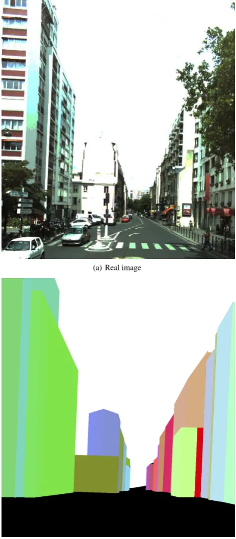
2. Perform a rasterization of the scene (see Fig. 1(b)) in a GPU buffer with a unique identifier per object of interest (Section 2.2).
(a) Real image
(b) Virtual image
Figure 1: A real image and superposable virtual image obtained by capturing the 3D model from the same point of view
2.1 Camera parameters transfer
Extrinsic parameters: Building an OpenGL camera simply re-quires to set the appropriate 4 by 4 matrix corresponding to the projective transform. However, special care should be taken as GPUs usually work in single precision floating point coordinates, as their development has always been driven by the games indus-try that focuses more on performance than on precision. This is completely incompatible with the use of geographic coordinates, and can lead to unacceptable imprecision during the rendering. A simple workaround is to choose a local frame centered within International Archives of the Photogrammetry, Remote Sensing and Spatial Information Sciences, Volume XXXVIII-3/W22, 2011
the 3D scene, in which both the 3D model coordinates and the camera orientation will be expressed.
Intrinsic parameters: Calibration of a camera sets its intrinsic parameters consisting mainly in its focal, principal point of au-tocollimation (PPA) and inner distortion. Conversely, OpenGL relies on the notion of field of view (FOV), the PPA is always at the perfect center of the image and distortion cannot be applied. In most cases, the PPA is close enough to the image center for this to be negligible. If it is not, a larger image should be cre-ated containing the image to be rendered and with its center at the PPA, then cropped. Finally, the field of view should then be be computed by:
F OV = 2.∗tan−1
max(width, height)
2f
; (1)
A simple means to handle the distortion is to resample the ren-dered image to make it finally perfectly superposable to the ac-quired one. Depending on the application, this resampling might not be necessary, and it might be more efficient to apply the dis-tortion on the fly when a visibility information is queried. In both cases, the width and height of the rendered image should be cho-sen such that its distortion completely encompasses the acquired image.
2.2 Rasterization
The problem ofrendering(generating virtual images of 3D scenes) has been widely studied in the computer graphics community, and two main methodologies have arisen:
1. Rasterizationconsists in drawing each geometric primitive of the scene using a depth buffer (also called Z-buffer) to know which primitive is in front of which from the current viewpoint.
2. Ray tracingconsist in intersecting each 3D ray correspond-ing to a screen pixel with the scene, then iteratcorrespond-ing on re-flected rays in order to define the appropriate color for that pixel.
Ray tracing is known to be much more expensive, but allows for very realistic lighting and reflexion effects. Ray tracing is also much harder to parallelize, such that GPUs always perform ren-dering by rasterization, making it extremely efficient and well suited in our case.
The result of a rasterization is a color image (the Z-buffer is also accessible if needed). Thus, the simplest way to get a visibility information from a rasterization is to give a unique color to each scene object of interest, and create a mapping between colors and scene objects. The only limitation to this method is that the num-ber of objects of interests should not exceed the numnum-ber of colors (2563
= 224
≈ 16.8million) which in practice is completely
sufficient (there are much less objects of interest such as facades or trees in the largest cities).
The second problem is that the size of the image to render might be arbitrarily larger than the size of the screen of the computer on which we will run the visibility computation. Hopefully, GPUs can performoffline rendering, that is to render a scene in a buffer of the GPU which size is only limited by the graphical mem-ory (GRAM). This buffer can then be transferred to the RAM, and saved on the disk if required. Using lossless compression is strongly advised as colors now have an exact meaning that should
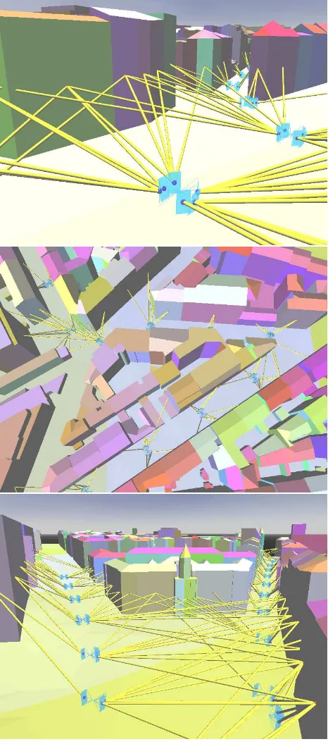
Figure 2: Set of images selected by our method as containing pertinent information about a facade (non wireframe)
absolutely be preserved, and most images rendered this way only present a limited number of colors arranged in large objects al-lowing for high lossless compression rates. In our experiments, the 1920x1080 buffers stored this way weighted 12 KBytes in average, which corresponds to a compression rate of 99.8%.
The result of this step, that we will callvisibility image(Fig. 1), stores the direct visibility information, i.e. the answer to the ques-tion: Which is the object seen at a given pixel of a given image? Some more work still needs to be done in order to answer effi-ciently to the image level question: which objects are seen well enough in a given image ? And the inverse one: which images see a given object well enough? The next section proposes a method to answer this questions that relies on a proper definition of the term ”well enough” in this context.
3 PICTURE LEVEL VISIBILITY
Most reconstruction/texture mapping problems can be decom-posed into one sub-problem for each scene element of interest. In this case, we need to be able to know which images will be useful to process the scene element in order to load them into the computer’s memory. Loading too many will impair processing time and memory footprint, but it can even lower the quality of the result in some cases. This section tackles these problems in two steps:
1. Defining geometric criteria to select which images are useful for the processing.
2. Building a visibility graph to answer to inverse visibility queries.
Optionally, we will propose two applications of the visibility graph structure:
1. Optimizing the memory handling in sequential treatment.
2. Selecting a single sequence to avoid limit issues due to non static scene elements (shadows, mobile objects,...).
3.1 Geometric criteria
The first naive approach to determining the scene elements seen in an image is simply to build a list of all colors present in a vis-ibility image, and declare the corresponding scene elements as viewed by the image. This is both inefficient and too simplistic. In fact, we want to select the images to use to process a scene ele-ment, so only the images seeing that element well enough should be used. Thus we propose two geometric criteria to select only the appropriate images:
1. Image content: The image should contain sufficient infor-mation about the scene element, or in other terms, the scene element should cover at least a certain portion of the visibil-ity image. This criterion also has a practical aspect: we can accelerate the color counting by only checking the colors of a small sparse subset of the image. For instance, if the cri-terion corresponds to 10 000 pixels, checking only every 1 000 pixel is sufficient, provided that the sampling is homo-geneous enough, and the criterion becomes having at least 10 samples of a given color. This will accelerate the pixel counting without impairing the result.
2. Resolution: The size of the pixel projected on the scene element should not exceed a given value (say25cm2) or a given multiple (say 5 times) of the smallest projected pixel size. We estimate this projected pixel size at the barycenter of the projection of the scene element in the visibility image (this can be done simultaneously to the color counting, us-ing the same sparse samplus-ing). This criterion penalizes both distance and bad viewing angles.
These criteria should be sufficient for most applications, but they can be adapted if needed. An example of the set of images se-lected for a given scene element (facade) based on these criteria is shown on Fig. 2.
3.2 The visibility graph
The geometric criteria cited above establish a relation: imageIi
sees elementEjwell enough, or conversely elementEjis seen in
imageIiwell enough. This relation is built from the image point
of view as for each image we define which elements are seen well enough. However, we usually need the inverse information: for the scene element on which we want to focus our method, which image should we use ? This requires to build a visibility graph containing two types of nodes (image and scene elements). Each visibility relation will be an edge in this graph between an image and an element node, that will be registered from both image and edge point of view. Constructing this graph is required to inverse the visibility information, but it is also useful for optimization and optionally for further simplification. A visualization of this visibility graph is proposed in Fig. 3.
Figure 3: Various views of the visibility graph computed on our test scene (for clarity, only10%of the images were used). Image (resp. scene) nodes are displayed in blue (resp. red).
3.3 Optimizing memory handling
The visibility graph allows to cut a reconstruction/texture map-ping problem into sub-problems by inputing only the images see-ing a scene element well enough. A trivial approach to process an entire scene sequentially is to load all these images when process-ing each scene element, then free the memory before processprocess-ing the next element. This trivial approach is optimal in terms of memory footprint, but an image seeingNscene elements will be loadedNtimes, which increases the overall computing time, es-pecially if the images are stored on a Network Attached Storage (NAS). Using a NAS is common practice in mobile mapping as International Archives of the Photogrammetry, Remote Sensing and Spatial Information Sciences, Volume XXXVIII-3/W22, 2011
Dataset #walls #images path length
Ours 4982 5344 (334x16) 1km
B´enitez 11408 1980 (990x2) 4.9km
Table 1: Comparison between our dataset and the dataset of B´enitez.
an acquisition produces around one TeraByte of (uncompressed) image data per hour. The optimization we propose is useful if the loading time is not negligible compared to the processing time, and if the network is a critical resource (in case images are on a NAS). It consists in finding the appropriate order in which to pro-cess the scene elements in order to load each image only once. The algorithm is based on the visibility graph, where additional information will be stored in each node (loaded or not for images, processed or not for scene elements):
1. Select any scene elementEjin the scene as starting point of
the algorithm and add it to a setSaof ”active elements”.
2. For each imageIij viewingEj, load it and add the
unpro-cessed elements seen byIj i toSa.
3. ProcessEj, markEjas processed and remove it fromSa.
4. If anIijhas all its viewed elements processed, close it.
5. Select the elementEjwith fewest unopened seeing images
inSa.
6. WhileSais not empty, go back to 2.
7. If no unprocessed element remain, terminate.
8. Select an unprocessed elementEjand go back to 2,
This algorithm is quite simple to implement once the visibility graph has been created, and will be evaluated in Section 4.
3.4 Sequence selection
Another useful utilization of the visibility graph issequence se-lection. In practice, we found out that images acquired by a mo-bile acquisition device are often redundant, as the coverage of an entire city require to traverse some streets more than once. Most georeferencing devices use an inertial central allowing for very precise relative localization but can derive due to GPS masks. Hence redundant image sequences viewing the same scene el-ement usually have a poor relative localization. Moreover, the scene may have changed between two traversals: parked cars gone, windows closed, shadows moved... In consequence, we propose to cluster the set of images seeing a given scene element according to their time of acquisition, then select the cluster (se-quence) with the best quality (using the criteria of Section 3.1).
4 RESULTS AND DISCUSSION
We have developed the tools described in this paper in order to perform large scale reconstruction and texture mapping of vari-ous urban objects such as facades, trees,... However, this paper only focuses on the optimized visibility computation, that is a mandatory prerequisite for such applications. Consequently, the results presented in this section consist mainly in statistics and timings demonstrating the quality efficiency of our approach.
The method presented in this paper (rasterization) was evaluated on a set of images acquired in a dense urban area with the mo-bile mapping system of (Bentrah et al., 2004). The set consists
Figure 4: Visualization of the 5344 images used in our experi-ments.
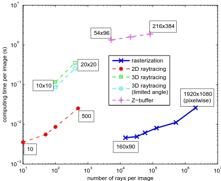
101 102 103 104 105 106 107 10−3
10−2 10−1 100 101
number of rays per image
computing time per image (s)
rasterization 2D raytracing 3D raytracing 3D raytracing (limited angle) Z−buffer 10x10
20x20
10
500 54x96
216x384
1920x1080 (pixelwise)
160x90
Figure 5: Timings for visibility computation. Results are com-pared between our rasterization approach (thick blue line) with subsampling factors ranging from 1 to 24, and the three ap-proaches of B´enitez (dotted lines).
of 334 vehicle positions, every 3 meters along a 1km path. For each position, 16 images were acquired (12 images forming a panoramic + 2 stereo pairs). We also disposed of a 3D city model of the acquired area built from aerial imagery. Comparison with the dataset of (B´enitez and Baillard, 2009) is displayed in Table 1. The main difference is that our path is shorter, but our im-age density is much higher. The imim-ages acquired are represented inserted in the 3D model on Fig. 4.
The timings for the computation of the visibility graph running on an NVidia GeForce GTX 480 are presented on Fig. 5, along with equivalent timings taken from (B´enitez and Baillard, 2009). They are given with respect to the number of visibility queries computed per image (number of rays traced or of buffer pixels). A high number of rays ensures that most visibility relationships will be found (good angular precision).
As expected, the use of the GPU allows for a huge performance increase for 3D visibility computation, even though our results are much more accurate: for an equivalent number of rays, our rasterization approach is around 400 times faster than Z-buffering. This huge performance increase is however limited to high ray numbers, as decreasing the resolution of our rasterization does International Archives of the Photogrammetry, Remote Sensing and Spatial Information Sciences, Volume XXXVIII-3/W22, 2011
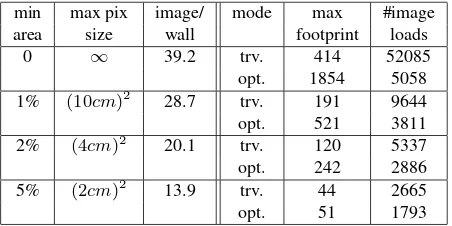
min max pix image/ mode max #image
area size wall footprint loads
0 ∞ 39.2 trv. 414 52085
Table 2: Influence of geometric criteria on visibility graph den-sity, and comparison of memory footprint and loading times be-tween trivial (trv.) and optimized (opt.) processing.
not improve the computing time below104
rays. Some steps of the rendering pipeline have a computation time depending on the number of primitives of the scene and not on the size of render-ing, which explains the limit we reach (around 4.6ms per image) for low resolutions. Even though our computing time does not improve below104
rays, it is still 20 times faster (for 160x90 rays) than 10x10 3D ray tracing.
The only method of (B´enitez and Baillard, 2009) with perfor-mance comparable to ours is 2D ray tracing. In our sense, this method is not suitable in urban areas in which configurations re-quiring the third dimension are often encountered (such as a taller building behind a smaller one). This is confirmed by (B´enitez and Baillard, 2009) who found that 2D ray tracing misses one third of the walls (compared to Z-buffering). Moreover, they state that 100 rays per image is a good compromise. For this number of rays, 2D ray tracing is already slower than our rasterization.
Finally, our approach is clearly the only one allowing for pix-elwise visibility computation in reasonable time (26ms per im-age, rightmost point of Fig. 5). It can even be brought down to 20ms per image with the color counting acceleration described in Section 3.1. This high performance makes pixelwise visibil-ity image computation time of the same order of magnitude than image loading time (15ms in our experiments), so the visibility images can be computed on the fly when required instead of be-ing precomputed and saved, which is another nice performance improving feature of our approach.
Finally, we evaluated the optimized memory handling by creating four visibility graphs of different densities by imposing increas-ingly harsh geometric constraints (see Table 2). As expected, op-timized processing greatly reduces the number of loads (each im-age is loaded exactly once) at the cost of memory footprint (maxi-mum number of images loaded simultaneously), and this effect is more important on denser graphs. If memory size is a limit and/or processing time is large compared to data loading time, then the trivial approach should be used. In other cases, and especially if data transfers are the bottleneck, then the optimized method will be preferable. Table 2 also shows that harsher constraints reduces the number of selected images, such that only the most pertinent ones are preserved.
5 CONCLUSIONS AND FUTURE WORK We have presented a methodology allowing easy scaling of recon-struction and texture mapping methods on large areas. Comput-ing the visibility graph of large scenes becomes tractable based on our approach, even at the pixel level. Enriching 3D models based on large amounts of data acquired at the ground level is becoming a major application of mobile mapping, and we believe that this methodology will prove useful to make the algorithms developed
in this context scalable. Our evaluation shows that our approach outperforms previous works both in quality and computing time.
The method described in this paper is mostly useful for texture mapping purposes where the per pixel visibility information is re-quired in order to predict occlusion of the model by itself. How-ever, it can also be used for unpredictable occlusions by insert-ing a point cloud correspondinsert-ing to detected occluders in the 3D scene before rendering. But this method can also be used for any reconstruction method where a rough estimate of the geometry is known (bounding box, point cloud, 2D detection in aerial im-ages,...)
In the future, we will look into optimizing our approach for larger 3D models based on spatial data structures such as octrees in or-der to load only the parts of the model that are likely to be seen. We will also investigate doing the color counting directly on the GPU to avoid transferring the buffer from graphics memory to RAM.
REFERENCES
B´enitez, S. and Baillard, C., 2009. Automated selection of ter-restrial images from sequences for the texture mapping of 3d city models. In: CMRT09. IAPRS, Vol. XXXVIII, Part 3/W4, pp. 97– 102.
B´enitez, S., Denis, E. and Baillard, C., 2010. Automatic produc-tion of occlusion-free rectified faade textures using vehicle-based imagery. In: IAPRS, Vol. XXXVIII, Part 3A (PCV’10).
Bentrah, O., Paparoditis, N. and Pierrot-Deseilligny, M., 2004. Stereopolis : An image based urban environments modelling sys-tem. In: International Symposium on Mobile Mapping Technol-ogy (MMT), Kunming, China, March 2004.
Frueh, C. and Zakhor, A., 2003. Constructing 3d city models by merging ground-based and airborne views. In: Proceedings of the 2003 IEEE Computer Society Conference on Computer Vision and Pattern Recognition (CVPR03).
Frueh, C. and Zakhor, A., 2004. An automated method for large-scale, ground-based city model acquisition. In: International Journal of Computer Vision, Vol. 60(1), pp. 5–24.
Haala, N., 2004. On the refinement of urban models by terrestrial data collection. Arch. of Photogrammetry and Remote Sensing, Commission III WG 7 35, pp. 564–569.
Huang, H., 2008. Terrestrial image based 3d extraction of ur-ban unfoliaged trees of different branching types. In: The Inter-national Archives of the Photogrammetry, Remote Sensing and Spatial Information Sciences, Vol. XXXVII, Beijing, China.
Korah, T. and Rasmussen, C., 2008. Analysis of building tex-tures for reconstructing partially occluded facades. In: European Conference on Computer Vision.
Lothe, P., Bourgeois, S., Dekeyser, F., Royer, E. and Dhome, M., 2009. Towards geographical referencing of monocular slam re-construction using 3d city models: Application to real-time accu-rate vision-based localization. In: IEEE Conference on Computer Vision and Pattern Recognition (CVPR’09), Miami, Florida.
P´enard, L., Paparoditis, N. and Pierrot-Deseilligny, M., 2004. 3d building facade reconstruction under mesh form from multiple wide angle views. In: IAPRS vol. 36 (Part 5/W17), 2005.
Wang, X., Totaro, S., Taillandier, F., Hanson, A. R. and Teller, S., 2002. Recovering facade texture and microstructure from real-world images. In: Proc. of the 2nd International Workshop on Texture Analysis and Synthesis in conjunction with ECCV’02, pp. 145–149.
Xiao, J., Fang, T., Zhao, P., Lhuillier, M. and Quan, L., 2009. Image-based street-side city modeling. In: ACM Transaction on Graphics, 28(5), 2009 (also in proceedings of SIGGRAPH ASIA’09).