T H E J O U R N A L O F H U M A N R E S O U R C E S • 45 • 3
and Wages
Evidence from Sweden and the United States
Illoong Kwon
Eva Meyersson Milgrom
Seiwoon Hwang
A B S T R A C T
This paper studies the long-term effects of the business cycle on workers’ future promotions and wages. Using the Swedish employer-employee matched data, we find that a cohort of workers entering the labor market during a boom gets promoted faster and reaches higher ranks. This pro-cyclical promotion cohort effect persists even after controlling for workers’ initial jobs, and explains at least half of the wage cohort effects that previ-ous studies have focused on. We repeat the same analyses using personnel records from a single U.S. company, and obtain the same qualitative re-sults.
I. Introduction
When the economy moves into a recession and the job market shrinks, both policymakers and workers are primarily concerned about the short-term consequences such as unemployment and wage cuts. However, a recession, even when temporary, can have long-term effects on workers’ careers. This paper shows that there exist strong procyclical cohort effects inpromotions. More
specif-Illoong Kwon is an assistant professor of economics at University at Albany, SUNY. Eva M Meyersson Milgrom is a senior scholar at Stanford Institute for Economic Policy Research and a visiting associate professor at Department of Sociology Stanford University. Seiwoon Hwang is a research fellow at Ko-rea Capital Market Institute. The authors are grateful to Ari Hietasalo, Svenskt Na¨ringsliv, A˚ ke Kempe, and Svenska Medlingsinstitutet for their extensive and exceptionally expert cooperation in preparing these data for analysis. We thank Bob Gibbons, Tor Ericsson, Guido Imbens, Edward Lazear, Paul Oyer, Katherine Shaw, Gary Solon, Michael Waldman, an anonymous referee, and participants of NBER Personnel Economics Meeting, Midwestern Economics Association Meeting, and Stanford GSB work-shop for helpful comments and suggestions. The data used in this article are from two confidential data sets. Researchers may contact the authors for further information at Eva M Meyersson Milgrom, SIEPR, 579 Serra Mall at Galvez Street, Stanford University, Stanford, CA 94305-6015.
[Submitted November 2008; accepted March 2009]
Kwon, Milgrom, and Hwang 773
ically, a cohort of workers who first entered the labor market during a recession gets promoted more slowly and reaches lower ranks than other cohorts, even after the recession is over. This effect persists even when we control for workers’ initial jobs. Most previous studies have focused on the effect of the business cycle on workers’ future wages and unemployment, but have paid relatively little attention to the effect on promotions, especially in the long run.1 However, promotions can have direct
effects on many aspects of workers’ careers and firms’ organization, including job assignments (Gibbons and Waldman 1999), human-capital accumulation (Prender-gast 1993), turnover (Kahn and Huberman 1988), authority (Aghion and Tirole 1997), communication (Friebel and Raith 2004), workers’ incentives (Lazear and Rosen 1981), and organizational rules and career mobility (Rosenbaum 1979a; Ro-senbaum 1979b; Spilerman 1986). Therefore, cohort effects in promotion imply that the business cycle can affect various aspects of workers’ careers and firms’ orga-nization structures over a much longer term than one may have thought.
Moreover, we find that cohort effects in wages are at least partially explained by cohort effects in promotions. In other words, workers who entered the labor market during a recession receive lower-than-average wages in the long run, largely because they get promoted more slowly and ultimately reach lower ranks than workers in other cohorts. As we will discuss later, these results imply that we need to reevaluate the theories of wage cohort effects as they do not necessarily explain the promotion cohort effects.
We use two data sources: the Swedish employer-employee matched data and the personnel records of a single U.S. firm. The Swedish employer-employee matched data cover almost the entire private sector from 1970 to 1990. These data build on a panel of personnel records of white-collar workers, and contain detailed rank and occupation information that iscomparable across firms. Thus, we can analyze pro-motion patterns of workers across thousands of firms for up to 20 years.
We complement the evidence from Sweden with a case study from a single oc-cupation in a single U.S. company. These U.S. data are based on personnel records of health insurance claim-processors in a large U.S. insurance company. Unlike the Swedish data, these U.S. data contain objective performance measures of each worker, so we can control for workers’ productivity directly.
Despite institutional differences between the United States and Sweden and the difference in scope between the two data sets, the qualitative results are remarkably similar: Both show strong procyclical cohort effects in promotions. Workers who entered the U.S. firm during a boom were promoted faster than average and reached higher-than-average ranks. Moreover, wage cohort effects are mostly driven by co-hort effects in promotions.
These results provide new insights into theoretical models of cohort effects. Re-cent theories have either emphasized the role of initial jobs and the productivity
differences among cohorts (Gibbons and Waldman 2006; Mroz and Savage 2006), or else have focused on long-term wage contracts (Beaudry and DiNardo 1991).
However, our results show that procyclical cohort effects persist even after control-ling for productivity and initial jobs, and that promotions, not necessarily wage itself, are responsible for the persistent cohort effects.
As far as we know, this is the first empirical study that analyzes cohort effects in both promotionsand wages. Moreover, our study is comparative, and incorporates two distinct data sets: (i) the representative Swedish data that cover an entire popu-lation of white-collar workers in the private sector over a 20-year period and (ii) the personnel records from a single U.S. firm that allow us to control for workers’ productivity objectively.
Earlier research has focused on cohort effects in wages using relatively small samples. For example, Freeman (1981), Oreopoulos, von Wachter, and Heisz (2006), and Kahn (2007) analyzed college graduates only. Baker, Gibbs, and Holmstro¨m (1994b) studied managers in a single U.S. firm. None of these studies controls for workers’ productivity.
Like this paper, Oyer (2006) studies the cohort effect in job ranking, but he focuses on the role of initial jobs among professional economists. He shows that new PhD economists who start at high-ranked departments are more likely to stay there in the future. Thus, entering the job market during a boom is better than entering during a recession because it is easier to find initial jobs at high-ranked departments during a boom. In contrast, we focus on cohort effects after controlling for initial jobs, and show that starting at a low-ranking job during a boom is still better than starting at the same low-ranking job during a recession. Solon, Whatley, and Stevens (1997) and Devereux (2000) study the influence of the business cycle on workers’currentjob assignments, and find that workers get assigned to lower-skilled jobs during a recession. In contrast, we focus on the influence of the business cycle on workers’futurejob assignments, as measured by the number of promotions and the speed of promotion.
Gibbons and Waldman (1999, 2006) provide a theoretical model where initial job placements and promotions play an important role in explaining cohort effects. We find partial support for their model. Though promotions do play a key role in our results, their model does not directly explain the remaining cohort effects on those who started at the same initial job.
II. The Swedish Employer-Employee Matched Data
The Swedish longitudinal data on white collar workers, an em-ployer—employee matched data set, covers the entire private sector of Sweden (ex-cluding banking and financial sectors) during the period 1970–90. For each worker, the data contain annual information on wage, age, education, gender, geographic region, work-time status, firm ID, plant ID, industry ID, and BNT codes (described below). Because all the IDs are unique, we can track each individual worker within and across firms throughout his/her career during 1970–90.Kwon, Milgrom, and Hwang 775
across firms. The Swedish employer-employee matched data are ideal in addressing this challenge because the BNT code allows just such a comparison.
The BNT code is a four-digit code, where the first three digits (called the occu-pation code) describe types of tasks and the fourth (called the rank code) describes the position’s degree of skill, as well as the number of subordinates available to fulfill the task. The white-collar workers’ occupations cover 51 three-digit occupa-tion groups such as construcoccupa-tion, personnel work, and marketing. (For more details, see Appendix 1.) Within each occupation, the rank code runs from 1 (lowest) to 7 (highest).2(For more details, see Appendix 2.)
The BNT codes served as the input to Sweden’s centralized wage negotiations, and were gathered and monitored by both The Swedish Federation of Employers and the labor unions. Thus, the occupation classifications have minimal measurement errors.3 Most importantly, the occupation and rank codes are comparable across firm. Thus, we can analyze workers’ promotion patterns for more than one firm, and even track what happens to workers who change firms. Few other data sets contain occupation and rank codes that are comparable across firms, and previous studies have thus focused on promotions within a single firm only (Baker, Gibbs and, Holmstro¨m 1994a,b).
Note that in contrast to the centralized wage negotiations, hiring and promotions were left to each employer’s own discretion. Thus, it is unlikely that the centralized wage bargaining system will affect the cohort effects in promotions directly. More-over, given that the centralized wage bargaining system put a great emphasis on equality, it should have reduced the cohort effects, because the cohort effects rep-resent the differences in wages and promotion rates among workers who are com-parable in every respect except for their labor market entry year (Meyersson Mil-grom, Petersen, and Snartland 2001). For more details on the data and the Sweden centralized wage bargaining system, see, for example, Ekberg (2004) and Calmfors and Forslund (1990).
In this study, we interpret a worker’s entry into our data as his/her first entry into the labor market.4We exclude those workers who already appear in the data in 1970
because we cannot observe their date of entry. Since we thus end up excluding most workers in the 1970s and early 1980s, we focus on the sample of workersbetween 1986 and 1989who have entered the data after 1970.5As shown, this selection also
makes the Swedish data more readily comparable to the U.S. data. Also, since the
2. Not every occupation spans all seven ranks: some start higher than one and some do not have the top ranks. Also the top executive managers (for example CEO) are not included.
3. Occupation classifications based on survey responses in other data are typically very noisy because workers often change their job description from year to year, even when they have not changed actual jobs (see Kambourov and Manovskii 2009).
4. Some workers may already have worked in the blue-collar market or in the public sector prior to entering our data. However, the private white-collar labor market is separate from other labor markets in that it is represented by separate labor unions and employer organizations. Thus, we ignore workers’ possible prior experience in other labor markets before entering our data.
Table 1
Age 1,024,856 36.9 24 36 51
Experience 1,024,856 6.73 1 6 14
Wage 1,024,856 11,721.32 7,100 11,000 17,200
Rank 1,024,856 3.36 1 3 5
Firm size 51,734 30.42 1 6 49
Note: The sample includes white-collar workers during 1986–89 who have first entered the data after 1970. Firm size is measured by the number of white-collar workers in a firm.
centralized wage-bargaining system began to dissolve after 1983, the wages are much more flexible during this sample period.
Table 1 shows the summary statistics of key variables. In a given year, on average, the data contain about 264,000 workers and 13,000 firms, yielding about one million individual-year observations, and 51,000 firm-year observations. On average, work-ers are 36.9 years old, and have 6.73 years of labor market experience.6 Their
average nominal monthly wage during 1986–89 is 11,721 Kronor, and the average rank (BNT) is 3.36, where Rank 1 is the lowest and Rank 7 is the highest. About 37 percent of workers are female, 19.61 percent have post-secondary education, and 13.18 percent are part-time workers.7About 11 percent of workers get promoted to
a higher rank every year, and in a given year 13 percent of workers are first-time entrants. Firm size is measured by the number of white-collar workers in the firm, and the average firm size is 30.42.
Figure 1 shows the fraction of workers in each rank, both for all workers, and for new entrants only. It is apparent that the rank structure is not a pyramid. Most workers are in Rank 3 or 4, and both the lowest rank and the highest rank contain a very small fraction of the workers. Figure 1 also shows that new entrants join the labor market at a wide range of ranks. Starting rank depends largely on education. Most college graduates enter at Rank 3 or 4, while most upper-secondary school graduates enter at Rank 2 or 3. Later we will estimate cohort effects separately for
Kwon, Milgrom, and Hwang 777
Figure 1
Rank Structure: Sweden
different education levels. Also, focusing on the subsample of workers whose start-ing rank is above Rank 3 does not change our results.8
III. Cohort Effects in Promotions
In this section, we estimate cohort effects in promotions, and study how they depend on the state of the business cycle at the time of workers’ first labor market entry.
A. Identification
For estimation of cohort effects in promotions, we regress workers’ current rank on a cohort dummy (cohortt), which is equal to one if a worker’s labor market entry year ist, and zero otherwise. As is well known, however, the coefficients of these cohort dummies, called the cohort effect in promotions, cannot be identified when we control for both labor market experience (henceforth experience) and year effects at the same time, because entry year is equal to year minus experience. However, as in McKenzie (2002), the nonlinear components of the cohort effects can be iden-tified.
More specifically, consider workeri with years of labor market experience at yeart. Suppose that the worker’s rank in yeartis determined as follows:
rank ⳱IⳭJⳭK
(1) it t tⳮ
whereItcaptures year effect;Jcaptures experience effect; andKtⳮ denotes labor market entry year (⳱tⳮ) cohort effects.
Suppose that there exists a linear trend that connects the first cohort effect and the last cohort effect in the sample with a slope of␣. Then, we can decompose the cohort effect as K ⳱␣(tⳮ)ⳭK⬘ , where K⬘ captures the nonlinear
compo-Note that Equation 2 holds for arbitrary␣. Thus, the linear trend in the cohort effects, ␣, cannot be identified.
As suggested by Hall (1971) and Berndt and Griliches (1995), however, we can still identify the nonlinear component of the cohort effects, K⬘ , by assuming
tⳮ
(namely, by dropping the first and the last cohort dummies in the regression). ␣⳱0
If this assumption (␣⳱0) is incorrect, the year and the tenure effects will be biased, but the nonlinear component of the cohort effects,Kt⬘ⳮ, or fluctuation around the linear trend, can still be correctly identified.9
8. The unreported robustness results in the paper are available from the authors.
Kwon, Milgrom, and Hwang 779
Figure 2
Identification of Cohort Effects: An Example
For example, suppose that in the true cohort effects, the linear trend that connects the first and the last cohort effect in the sample has positive slope, ␣⬎0, as in Figure 2a. Though we cannot identify the slope ␣, dropping the first and the last cohort dummies in a regression identifies the nonlinear component,K⬘ , as shown
in Figure 2b. Since we are interested in the effect of the business cycle (or the economy’s fluctuation around a possible linear growth trend) on cohort effects, the identification of nonlinear components in cohort effects is sufficient for our pur-pose.10
To improve efficiency, we also control for experience using a polynomial function of experience, instead of experience dummies. Using experience dummies, however, does not change the qualitative results of our analysis.
Another identification problem is the possible endogeneity of labor market par-ticipation. For example, during a recession, workers may delay participating in the labor market, perhaps opting for additional education instead (see Raaum and Røed 2006). If this endogenous decision affects the average productivity of each cohort, it could generate a bias in our estimation.
In our analysis of the Swedish data, we argue that the direction of potential bias will not change the interpretation of our results. In the analysis of the U.S. personnel data, we control for workers’ productivity directly, and demonstrate that the direction of potential bias in fact strengthens our interpretation.
B. Procyclical Cohort Effects
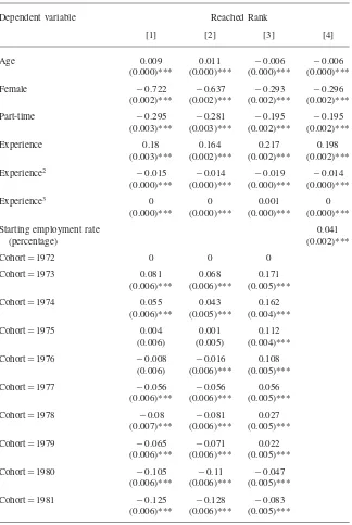
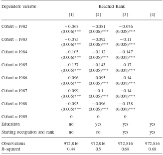
In Table 2, we regress workers’ rank on age, gender, part-time dummy, firm size, and annual firm-size growth rate, as well as a polynomial of experience, cohort dummies, year-dummies, 31 industry dummies, 49 occupation dummies (the first three digits of the BNT code), and 24 regional dummies.
Even though rank is not a continuous variable, for easy interpretation, we treat it as a linear variable for our analyses. However, using ordered-probit regression does not change any qualitative results of this paper.
Column 1, Table 2, shows that different cohorts of workers ultimately reach dif-ferent ranks, even after controlling for basic individual characteristics including ex-perience. For example, workers who entered the labor market in 1973 reached ranks about 0.2 higher than workers who entered the labor market in 1985. Given that there are only seven ranks and that the average annual promotion rate is 11 percent, this difference is economically significant.11
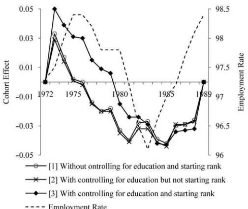
Figure 3 illustrates the estimated cohort effects in Table 2 along with the em-ployment rate (⳱ 100 ⳮ unemployment rate) at the time of entry. For example,
Line 1 in Figure 3 shows the cohort effects estimated in Column 1, Table 2. The correlation between cohort effects (Line 1) and employment rates is 0.39. Therefore,
cohort effects in promotion are procyclical. In other words, workers who entered the labor market during a boom reach higher ranks in the future, even after con-trolling for individual characteristics, including experience.
An important concern is that procyclical cohort effects on promotion might arise if the average productivity of cohorts who entered during a boom is higher than that of other cohorts. However, our analysis suggests just the reverse. In Column 2, Table
10. Allowing for quadratic trends in cohort effects does not change our results.
Kwon, Milgrom, and Hwang 781
Experience3 0 0 0.001 0
(0.000)*** (0.000)*** (0.000)*** (0.000)***
Cohort⳱1973 0.081 0.068 0.171
(0.006)*** (0.006)*** (0.005)***
Cohort⳱1974 0.055 0.043 0.162
(0.006)*** (0.005)*** (0.004)***
Cohort⳱1975 0.004 0.001 0.112
Table 2(continued)
Starting occupation and rank no no yes yes
Observations 972,816 972,816 972,816 972,816
R–squared 0.44 0.5 0.68 0.68
Note: Standard errors are in parentheses. * significant at 10 percent; ** significant at 5 percent; *** significant at 1 percent. The dependent variable is the workers’ rank in 1986–89. Each regression includes firm size, annual firm size growth rate, female, part-time, 31 industry, 49 occupation, 24 county, and 3 year dummies. “cohort⳱t” is equal to one if a worker’s labor market entry year is equal tot, and zero otherwise. cohort⳱1972 and cohort⳱1989 are set to zero for identification as discussed in the text. Edu-cation is controlled by six eduEdu-cation dummies (elementary, lower-secondary, upper-secondary, bachelor, master, and PhD). Starting rank and current rank are controlled by seven rank dummies (1–7). The coef-ficients of cohort effects in Column 1, 2, and 3 are also shown in Figure 2.
2, we first control for workers’ education as a proxy for workers’ productivity. As Figure 3 shows, controlling for education makes little difference in cohort effects.
Kwon, Milgrom, and Hwang 783
Figure 3
Cohort Effects in Reached Rank: Sweden
Note: This figure shows the estimated coefficients of cohort dummies in Table 2, Columns 1, 2, and 3 along with the employment rates (⳱100-unemployment rate in percentage).
during recessions (Clark and Summers 1981; Devereux 2002), controlling for work-ers’ initial jobs should increase the magnitude of cohort effects.
Line 3 in Figure 3 shows that controlling for workers’ initial jobs increases the magnitude of cohort effects. For example, compared with Line 1 where we don’t control for education or initial jobs, the difference in reached rank between the 1973 cohort and the 1985 cohort increases from 0.2 to 0.3, and the correlation between cohort effect and employment rate increases from 0.39 to 0.57.
These results imply that the average productivity of cohorts who entered the labor market during a boom is lower (not higher) than that of other cohorts. That is, the procyclical cohort effects in promotions are not necessarily driven by the different productivities of each cohort. Furthermore, later we can show that when we control for workers’ productivity directly in the U.S. data, the cohort effects in promotion still remain procyclical.
Column 4, Table 2, controls directly for the employment rates when workers entered the labor market, instead of controlling for cohort dummies. As expected, the correlation between employment rates and ranks is positive and highly signifi-cant. For example, a one percent point increase in the employment rate at the time of labor market entry will lead to a rank 0.4 higher in the long run.
1970s as our estimated cohort effects closely follow the actual business cycle in the 1970s.
These procyclical cohort effects in promotions are more surprising than the cohort effects in wages: given that promotions affect job assignment, human capital accu-mulation, productivity, and profit more directly than wages do, it is puzzling that firms seem to allow the business cycle at the time of workers’ labor market entry to affect their future promotion decisions.
Also note that controlling for workers’ initial jobs (or their first occupations and ranks) increases both the magnitude of the estimated cohort effects and their cor-relation with employment rates. That is, even those who started their careers in the same job may end up at different ranks depending on the business cycle at the time of their labor market entry.12Therefore, these findings cannot be fully explained by
previous studies that have focused on the effect of workers’ initial jobs on their future careers (Gibbons and Waldman 2006; Oyer 2006). We will discuss the theo-retical implications of promotion cohort effects in greater detail in the last section.
IV. Cohort Effects in Wages
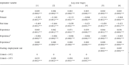
In this section, we estimate cohort effects in wages in Sweden, using the same specification as in Table 2, except that the dependent variable is now log(real wages) instead of rank.
Column 1, Table 3, gives estimates of the cohort effects in wages without con-trolling for workers’ education and initial jobs. Figure 4a illustrates that these cohort effects (Line 1) are approximately procyclical. For example, the correlation between the wage cohort effect and the employment rates is 0.48. The cohort-driven wage differential is economically significant: workers who entered in 1973 receive 7.5 percent higher wages than those who entered in 1985, even after controlling for various individual characteristics, including experience.
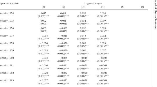
In Columns 2 and 3, Table 3, we also control for workers’ education and their initial jobs. As with the cohort effects in promotions, Figure 4a shows that control-ling for education does not make much difference, and that controlcontrol-ling for workers’ initial jobs makes the magnitude of cohort effects even larger, not smaller. For example, compared with Line 1 where neither education nor initial jobs are con-trolled for, the wage difference between the 1973 cohort and the 1985 cohort in-creases from 7.5 percent to 9.3 percent and the correlation with employment rates increases from 0.48 to 0.60. These results again suggest that initial job ranks cannot fully account for the procyclical cohort effects in wages.
Unlike previous studies, we also control, in Column 4, Table 3, for workers’ current rank. Figure 4b shows that wage cohort effects decrease significantly when we control for workers’ current rank. For example, the wage difference between the 1973 cohort and the 1985 cohort decreases from 7.5 percent to 3.6 percent.
For easier interpretation, in Columns 5 and 6, Table 3, we control for employment rates at the time of workers’ labor market entry, instead of using cohort dummies.
Kwon,
Milgrom,
and
Hwang
785
Table 3
Cohort Effects in Wages: Sweden
dependent variable Log (real wage)
[1] [2] [3] [4] [5] [6]
Age 0.005 0.006 0.002 0.003 0.002 0.003
(0.000)*** (0.000)*** (0.000)*** (0.000)*** (0.000)*** (0.000)***
Female ⳮ0.202 ⳮ0.180 ⳮ0.113 ⳮ0.068 ⳮ0.114 ⳮ0.068 (0.001)*** (0.001)*** (0.001)*** (0.000)*** (0.001)*** (0.000)***
Part-time ⳮ0.469 ⳮ0.466 ⳮ0.450 ⳮ0.421 ⳮ0.450 ⳮ0.421 (0.001)*** (0.001)*** (0.001)*** (0.001)*** (0.001)*** (0.001)***
Experience 0.065 0.062 0.071 0.039 0.064 0.036
(0.001)*** (0.001)*** (0.001)*** (0.000)*** (0.001)*** (0.000)***
Experience2 ⳮ0.006 ⳮ0.006 ⳮ0.006 ⳮ0.004 ⳮ0.005 ⳮ0.003 (0.000)*** (0.000)*** (0.000)*** (0.000)*** (0.000)*** (0.000)***
Experience3 0.000 0.000 0.000 0.000 0.000 0.000
(0.000)*** (0.000)*** (0.000)*** (0.000)*** (0.000)*** (0.000)***
Starting employment rate 0.011 0.005
(0.000)*** (0.000)***
Cohort⳱1972 0 0 0 0
Cohort⳱1973 0.033 0.029 0.050 0.023 (0.002)*** (0.002)*** (0.001)*** (0.001)***
The
Journal
of
Human
Resources
Table 3(continued)
dependent variable Log (real wage)
[1] [2] [3] [4] [5] [6]
Cohort⳱1974 0.017 0.014 0.039 0.014 (0.002)*** (0.001)*** (0.001)*** (0.001)***
Cohort⳱1975 0.002 0.001 0.031 0.019 (0.001) (0.001) (0.001)*** (0.001)***
Cohort⳱1976 0.000 ⳮ0.002 0.030 0.018 (0.002) (0.002) (0.001)*** (0.001)***
Cohort⳱1977 ⳮ0.014 ⳮ0.015 0.015 0.012 (0.002)*** (0.002)*** (0.001)*** (0.001)***
Cohort⳱1978 ⳮ0.020 ⳮ0.020 0.009 0.009 (0.002)*** (0.002)*** (0.002)*** (0.001)***
Cohort⳱1979 ⳮ0.018 ⳮ0.020 0.006 0.007 (0.002)*** (0.002)*** (0.001)*** (0.001)***
Cohort⳱1980 ⳮ0.033 ⳮ0.035 ⳮ0.015 ⳮ0.003 (0.002)*** (0.002)*** (0.001)*** (0.001)***
Cohort⳱1981 ⳮ0.040 ⳮ0.041 ⳮ0.024 ⳮ0.008 (0.002)*** (0.002)*** (0.001)*** (0.001)***
Cohort⳱1982 ⳮ0.028 ⳮ0.032 ⳮ0.024 ⳮ0.008 (0.002)*** (0.002)*** (0.001)*** (0.001)***
Kwon,
Milgrom,
and
Hwang
787
Cohort⳱1984 ⳮ0.039 ⳮ0.041 ⳮ0.042 ⳮ0.015 (0.001)*** (0.001)*** (0.001)*** (0.001)***
Cohort⳱1985 ⳮ0.042 ⳮ0.044 ⳮ0.043 ⳮ0.013 (0.001)*** (0.001)*** (0.001)*** (0.001)***
Cohort⳱1986 ⳮ0.030 ⳮ0.029 ⳮ0.034 ⳮ0.010 (0.001)*** (0.001)*** (0.001)*** (0.001)***
Cohort⳱1987 ⳮ0.029 ⳮ0.029 ⳮ0.033 ⳮ0.010 (0.001)*** (0.001)*** (0.001)*** (0.001)***
Cohort⳱1988 ⳮ0.026 ⳮ0.027 ⳮ0.032 ⳮ0.009 (0.001)*** (0.001)*** (0.001)*** (0.001)***
Cohort⳱1989 0 0 0 0
Education no yes yes yes yes yes
Starting occupation and rank no no yes yes yes yes
Current rank no no no yes no yes
Observations 972,816 972,816 972,816 972,816 972,816 972,816
R–squared 0.61 0.65 0.73 0.81 0.73 0.81
Figure 4
Cohort Effect in Wages: Sweden
Kwon, Milgrom, and Hwang 789
Figure 5
Wage Dispersion and Rank: Sweden
Note: Distribution of nominal monthly wages in 1988 for occupation 310 (mechanical engineering) and occupation 800 (marketing). The rectangular box represents the 25th percentile to 75th percentile range.
Column 5 shows that employment rates at the time of entry have a large and sig-nificant effect on current wages. However, once we control for workers’ current ranks, the effect on wages of employment rates at the time of entry decreases by more than 50 percent.
The decrease in the significance of wage cohort effects when we control for rank suggests that cohort effects in wages are at least partially driven by cohort effects in promotions: workers who entered the labor market during a boom receive larger-than-average wages in the long run partially because they get promoted to higher-than-average ranks, even after controlling for their initial jobs.
These results would not be surprising if a single wage were tied to each rank, because then a firm could not raise workers’ wages without promoting them. How-ever, as Figure 5 shows, there exist large wage variations even within each rank. In particular, wage distributions overlap across different ranks. Thus, some workers in lower ranks receive larger wages than those in higher ranks.13
Also, controlling for current rank has a relatively small effect on overall fit, in-creasing the wage-regressionR-squared by less than ten percent of a point (see Table 3, Column 3, to Table 3, Column 2).
Many studies have shown that a significant proportion of wage increases over a career are tied to promotions (Lazear 1992; Baker, Gibbs, and Holmsto¨m 1994b; McCue 1996). As far as we know, though, this is the first empirical study to show
Figure 6
Cohort Effects in Promotions by Gender: Sweden
that a significant part of cohort effects in wages is driven by cohort effects in pro-motions.
As will be discussed in Section VII, these findings also provide important insights into the theories of cohort effects because many existing theoretical models cannot explain broad patterns of our findings.
V. Heterogeneity in Cohort Effects
In this section, we analyze how cohort effects in promotions vary across different groups of workers. We find that cohort effects are nearly constant across gender and education levels, but that heterogeneity exists across occupations. Previous studies were based on relatively small or homogeneous samples, and could not analyze such heterogeneity.
A. Gender
In Figure 6, we illustrate the cohort effects in promotions estimated separately for each gender, controlling for both education and starting rank. The regression spec-ification is the same as that in Table 2, Column 3.
Kwon, Milgrom, and Hwang 791
Figure 7
Cohort Effects in Promotions by Education: Sweden
B. Education
In Figure 7, we illustrate the cohort effects in promotion estimated separately for each education group.14Again, the specification of the regression is the same as that
in Table 2, Column 3. Sweden has a nine year compulsory school program for all children between the ages of 7 and 16 years, equivalent to a tenth grade education in a U.S. high school. This can be followed by between two and four years of upper-secondary, and then further postsecondary education. In 1988, 60 percent of workers in our sample had the compulsory education degree only, 20 percent had an upper-secondary degree, and 20 percent had a postupper-secondary education degree.
Figure 7 shows that the cohort effects in promotions for each education group are all procyclical. The correlation with the employment rate is 0.55 for the compulsory, 0.56 for the upper-secondary, and 0.56 for the post-secondary education group. The magnitude of cohort effects is quite similar between compulsory and post-secondary education groups. The cohort effects for the upper-secondary education group are somewhat smaller than the others, especially in the 1970s.
While previous studies suggest that low-skilled workers are more susceptible to the effects of the business cycle (see, for example, Hoynes 2000), our results suggest that the long-term effect of the business cycle (at the time of labor market entry) is relatively constant across education levels. This result is consistent with the finding
that controlling for education does not make much difference in the estimation of cohort effects in promotions (Table 2) and wages (Table 3).
B. Occupation
Finally, we estimate the cohort effects in promotions by one-digit occupation groups. At the one-digit level, there are ten occupation groups (see Appendix 1). Among these, we focus on six groups, omitting the four smallest occupation groups.
As illustrated by Figure 8, all occupations demonstrate procyclical cohort effects in promotions, as well as correlations larger than 0.45 with the employment rate. However, Figure 8 reveals the differences in the magnitudes of cohort effects across occupations. Workers in financial work and office service have the largest cohort effects. The difference between the 1975 cohort and the 1985 cohort is 0.4 rank. As discussed above, given that there are only seven ranks and that the annual promotion rate is 11 percent, a 0.4 rank-difference driven only by the business cycle at the time of entry is quite large. Workers in production management, by contrast, have the least-significant cohort effects: the difference between the 1974 cohort and the 1985 cohort is only 0.15 rank.
The analysis of underlying causes for this heterogeneity across occupations is beyond the scope of this paper, but certainly is an interesting and important question for future research.
VI. Evidence from the United States
In this section, we complement the evidence from Sweden with a case study of a single occupation in a single U.S. firm. The U.S. data are based on personnel records of health insurance claim processors in a U.S. insurance firm. As we describe below, these U.S. data are not directly comparable to the Swedish data: still, they complement the Swedish data in several respects.
First, these U.S. data contain an objective performance measure of each worker, allowing us to control for workers’ productivity directly. Second, the ranks in this group of workers are much narrower than those in the Swedish data, and can thus be considered equivalent to subranks within a rank in Sweden, allowing us to analyze smaller-scale promotions that the Swedish data may not capture. Third, because this is a U.S. company, the results serve as evidence that the findings in Sweden can be generalized to other countries.
A. The U.S. Data
The data, from the personnel records of health-insurance claim processors in a large U.S. insurance company, include information on 3,231 full-time indemnity claim-processors over a two-and-a-half-year period (01/01/93–06/30/95). Among these, we focus on the 2,750 workers hired after 1984.15Note that, unlike in the Swedish data,
Kwon, Milgrom, and Hwang 793
Figure 8
Cohort Effects in Promotions by Occupation Group: Sweden
we cannot observe each worker’s entire wage history; still, we can observe when they were hired and the condition of the economy at the time of hire.
Table 4
Summary Statistics of U.S. Personnel Data
Observations Mean
Wage (six month sum) 8,766 10,285 8,050 9,593 12,542
Rank 8,766 2.12 1 2 4
Tenure 8,766 3.78 1 3 8
Female 8,766 91.8
Post secondary education 8,766 33.4
Performance 8,766 162.52 53.28 149.7 276.15
Note: Female and post secondary education are in percentage. Performance measures the average daily performance.
including salary, bonuses, and overtime payment, and (iii) individual characteristics including gender, marital status, age, and hiring date.16The data also contain
work-ers’ job numbers to distinguish the types of claims they process. For simplicity, we use six-month average measures throughout the analysis.17Table 4 provides
sum-mary statistics of selected variables.
About 92 percent of the employees are female, and 58 percent are married. The average age is 30 years. Most of the employees have high school diplomas, and about 30 percent of them have a college education or higher. The average six-month nominal wage is about $10,285.
The workers’ tasks involve computer data-entry of insurance claims, which re-quires knowledge of medical terminology and various codes. Therefore, despite the simple nature of the task, there exists a significant learning-by-doing curve for the first five years of tenure. For example, for the first six months, a worker typically processes 85 claims per day, but after five years, a typical worker can process more than 200 claims per day. On the whole, these employees can be characterized as female, nonmanagerial, white-collar, full-time, service-industry workers.
It is worth emphasizing that the performance measure, namely the weighted num-ber of claims processed per day, reflects the workers’ productivity accurately, be-cause (i) these workers do not perform any other tasks; (ii) different types of claims processed in different ranks are adjusted by the weighting system that the company developed; and (iii) the company itself relies on this performance measure in wages and promotion decisions. Therefore, we can directly control for possible productivity differences among different cohorts.
16. In measuring workers’ performance, the company developed its own‘weighting system’ to take into account different types and difficulties of claims.
Kwon, Milgrom, and Hwang 795
Mobility in this job is very high. About 32 percent of the workers leave the firm during the two-and-a-half-year sample period, and tenure, measured as the number of years since the date of hire, is thus relatively short.
Using a transition matrix of job numbers, as in Baker, Gibbs, and Holmstro¨m (1994a), we can identify four different hierarchical ranks within this firm and oc-cupation, with 1 being the lowest and 4 the highest. Rank 1 is most common (48 percent), and the fractions of workers in Rank 2 and above are nearly the same (about 17 percent each).
All new workers start at the bottom rank and are promoted to higher levels based on tenure and performance. The ranks differ mainly in the types of claims the workers process. In general, higher ranks involve more complicated and technical claims than lower ranks. But since the basic nature of the tasks is the same, these U.S. ranks can be considered as subranks within a given Swedish BNT rank. For more details on the U.S. data, see Kwon (2006).
B. Cohort Effects in Promotions and Wages in the U.S. Data
To estimate cohort effects in promotions, we regress workers’ job ranks18on their
performance, tenure, tenure squared, years of education, gender, and marital status, as well as time dummies, three-digit zip code dummies, and cohort dummies. Again, time and cohort are measured in six-month units (for example, 1985–1, 1985–2, 1986–1, . . .). As before, we drop the first and the last cohort dummies in order to identify the fluctuation of cohort effects over the possible linear trend.
Note that, in these U.S. data, we analyze cohorts of workers who entered thefirm
in the same year, not those who entered thelabor marketin the same year. However, given that all workers start at the lowest rank and learn from scratch, differences in prior labor market experience may be irrelevant. And the Swedish data support this assumption: redefining cohorts as those who entered a firm in the same year and repeating the entire analysis does not change the qualitative results.19
Figure 9 illustrates the estimated cohort effects in promotions. Like those in Swe-den, the cohort effects in promotions in this U.S. firm are highly procyclical. Their correlations with the employment rates are 0.53 without controlling for productivity, and 0.56 controlling for productivity. The magnitude of these cohort effects is also large: workers who entered this firm in 1989 (during a boom) get promoted to 0.5 rank higher than the comparable workers who entered in 1993 (during a recession). Given that there are only four ranks, this difference is significant.
Not surprisingly, Column 1, Table 5, shows that the employment rate at the time of labor market entry has a significant and positive effect on current ranks.
Unlike the Sweden case, we can also control for workers’ productivity directly in this U.S. sample. It is important to note that controlling for productivity yields very little change in the estimated cohort effects: if anything, it makes the magnitude of cohort effects even larger. For example, from Figure 9, the difference between the 1989 cohort and the 1993 cohort increases from 0.5 to 0.55 rank after controlling
Figure 9
Cohort Effects in Promotions: U.S. Personnel Data
for performance. This result supports our earlier argument that differences in the average productivity of each cohort cannot fully explain the procyclical cohort ef-fects.
Figure 10 also show the estimated cohort effects in wages. Lines 1 and 2 show that the overall patterns of cohort effects in wages are similar to those of cohort effects in promotions. First, wage cohort effects are very procyclical. For example, the correlation between the cohort effects (Line 1) and employment rate is 0.51. Second, controlling for performance does not explain the procyclical cohort effects. Furthermore, as in the Sweden case, Line 3 in Figure 10 shows that controlling for workers’ current ranks significantly diminishes the cohort effects in wages, nearly eliminating, for example, the difference between the 1989 and 1993 cohorts, and decreasing the correlation with employment rate from 0.51 toⳮ0.04.
Alternatively, in Columns 2 and 3, Table 5, we control for the employment rate when the worker was initially hired, instead of using cohort dummies. Without controlling for workers’ current rank, the initial employment rate has a strong and significant effect on workers’ current wages. However, once we control for workers’ current rank, the effect of initial employment rate decreases substantially, from 0.016 to 0.004. Thus, procyclical cohort effects inwages in this U.S. firm are explained largely by procyclical cohort effects inpromotions.
Kwon, Milgrom, and Hwang 797
Table 5
Cohort Effects in Promotions and Wages: U.S. Personnel Data
Dependent variable Rank Log(wage)
Tenure squared ⳮ0.01 ⳮ0.001 0
(0.000)*** (0.000)*** (0.000)***
Note: Standard errors are in parentheses. * significant at 10 percent; ** significant at 5 percent; *** significant at 1 percent. In Column 1, the dependent variable is the workers’ rank in 1993–95. In Columns 2 and 3, the dependent variable is the log real wage. Each regression also includes female, marital, time, and zip code dummies. Employment rate is measured in the year when workers first enter the data. Edu-cation is measured by years of eduEdu-cation. Performance is measured by six-month average performance. Tenure is measured by a six-month unit. For example, tenure⳱2 is equivalent to one year. Starting ranks are not controlled because everyone in this firm starts from Rank 1.
One must be careful in drawing quick conclusions from this comparison between Sweden and the United States because the data sets are very different. For Sweden, we used representative employer-employee matched data encompassing 56 broad occupation groups and thousands of firms. For the United States, we used a specific occupation group in a single company. But the similarity in results is striking nev-ertheless.
VII. Discussion
Figure 10
Cohort Effects in Wages: U.S. Personnel Data
Figure 11
Wage Dispersion and Rank: U.S. Personnel Data
Kwon, Milgrom, and Hwang 799
A. Productivity-Based Theories of Cohort Effects
Though our results suggest that promotion cohort effects, not necessarily productiv-ity, drive wage and unemployment cohort effects, it is nevertheless important to consider productivity differences among different cohorts, which may arise for vari-ous reasons:
1. Initial Jobs and Learning
Gibbons and Waldman (2006) suggests that, during a boom, new workers get as-signed to higher-ranked jobs where they can learn more valuable task-specific, skills. They thus become more productive, receive larger wages, and get promoted faster than those who enter during a recession. Oyer (2006), for example, suggests that new economists hired at high-ranked departments may have more research time and more interaction with successful colleagues, which can lead to faster growth in research productivity.
Such models, however, cannot explain why procyclical cohort effects persist after controlling for initial jobs (in Sweden), and even after controlling for productivity (in the United States).20
One could argue that the ranks in the Swedish data are too coarse and noisy measures of workers’ true rank. If that is true, then cohort effects should remain even after controlling for initial ranks. In such a case, controlling for initial ranks should still reduce the size of cohort effects. Recall, however, that as discussed in Sections III and IV, controlling for workers’ initial ranks and occupations does not reduce the magnitude of cohort effects, rather, it increases it slightly. This result suggests that the measurement errors in the rank variable are not responsible for the cohort effects remaining after controlling for initial ranks.
2. Procyclical Matching Quality
The quality of workers’ matches with their initial jobs directly affects productivity. Since better-matched workers are less likely to change jobs and thus less likely to lose firm- or task-specific human capital, they will have higher-than-average pro-ductivity in the long run, receive larger wages, and reach higher ranks than poorly-matched workers. But there exist two contrasting theories that relate the business cycle to match quality.
The first suggests that, since more jobs are available during a boom than during a recession, it can be easier for new workers to find better-matched jobs during a boom (Gan and Li 2004). The second, however, suggests that, since there are more workers seeking jobs during a recession than during a boom, firms can find better-matched (or higher productivity) workers during a recession (Clark and Summers 1981).
Our results from the Swedish data suggest that the productivity of cohorts who entered during a recession appears to be higher than the average, and support the
latter theory. However, the latter theory predicts counter-cyclical cohort effects, not procyclical cohort effects, and neither theory can explain why procyclical cohort effects persist even after controlling for productivity in the U.S. data.
In fact, it is somewhat surprising that controlling for productivity in the U.S. data does not explain the cohort effects much, as illustrated in Figure 9. Even though we cannot definitely rule out the productivity-based theories, our results suggest that the productivity differences among different cohorts cannot fully explain the procyclical cohort effects.
B. Nonproductivity-Based Theories of Cohort Effects
So far, we have discussed theories of cohort effects based on differences in produc-tivity. The other set of theories suggests several other factors, none fully satisfactory, that might drive the observed cohort effects:
1. Downward Rigidity
Previous studies using both U.S. and Swedish data show that both demotions and nominal wage-cuts are very rare (Baker, Gibbs, and Holmstro¨m 1994a; Agell and Lundborg 2003; Kwon and Meyersson Milgrom 2008). Such downward rigidity can arise, for example, if firms and workers cannot apply termination of the employment relationship as an effective threat in their bargaining (Hall and Milgrom 2008). If workers start at higher ranks (or receive larger wages) during a boom, then down-ward rigidity ensures that in the future they will, on average, still be in a higher rank (or receive larger wages) than those who started during a recession.
This explanation may account for cohort effects in the short run, but it is unlikely to explain rank and wage gaps that persist as much as 17 years after entry, as observed in Sweden; even if firms can’t demote workers or cut wages, they can slow down promotions if workers hired during a boom were assigned to higher-than-usual ranks initially. Using the Swedish data, we estimate the cohort effects in promotion speed, where promotion speed is measured by number of promotions divided by experience.21The effect of downward rigidity should lead us to expect
counter-cyclical cohort effects in promotion speed. But Figure 12 shows that cohort effects in promotion speed are still procyclical.
These procyclical cohort effects in promotion speed are particularly important because they suggest that the rank and wage gaps between a boom cohort and a recession cohort won’t shrink, but rather will increase (or at least persist) in the long run.
2. Signaling or Stigma
As Waldman (1984) emphasizes, job assignment can be a strong signal of a worker’s productivity. In particular, Oyer (2006) suggests that the labor market can take the initial job as a signal for a worker’s ability without fully discounting the luck as-sociated with the business cycle at the time of entry. In other words, the low rank
Kwon, Milgrom, and Hwang 801
Figure 12
Cohort Effects in Promotion Speed: Sweden
Note: The figure shows the cohort effects in promotion speed (⳱number of promotions divided by experience). The regression specifications are the same as in Columns 1 and 2, Table 2, except that the dependent variable is now promotion speed.
of the initial jobs new workers have to accept during a recession can stigmatize them and hamper their careers.
Again, though, this model cannot explain why procyclical cohort effects persist (and even increase) after controlling for initial jobs in Sweden. Moreover, the U.S. analysis is based on those who started at the same firm and the same job level, but still reveals strong procyclical cohort effects.
3. Long-Term Contracts
Risk-averse workers who sign a long-term contract during a recession may be willing to accept lower long-term wages than those who sign a contract during a boom. With some friction in mobility (such as moving-cost or loss of specific skills), such a long-term contract can generate procyclical cohort effects in wages (Beaudry and DiNardo 1991), though this model, too, does not directly explain cohort effects in promotions.
effects offered by the long-term-contract model and an extended version of Gibbons and Waldman (2006) with multiple periods where the job assignment in early pe-riods, not just the first job assignment, determine the future promotions and wages.
VIII. Conclusion
This paper shows that workers who enter the labor market during a boom are promoted faster and reach higher ranks than those who enter during a recession. These findings suggest that the business cycle can have long-term effects in the labor market by affecting new workers’ promotion and job-assignment pros-pects, which in turn affect workers’ incentives and firms’ performance. Our analysis also suggests that thewagecohort effects previously addressed in the literature are at least partially explained by thesepromotioncohort effects.
At the same time, these findings present new puzzles: differences in the rankings of initial jobs cannot explain these cohort effects, since starting at a low-ranked job during a boom is still better than starting at the same low-ranked job during a recession. Nor can cohort effects be fully explained by productivity differences among different cohorts, whether due to difference in initial-job rank, worker-job match quality, or on-the-job human-capital investment. Investigating the sources of these promotion cohort effects will be an interesting topic for future research, and we suspect that the observed heterogeneity in the magnitude of cohort effects across different occupations will yield an important clue.
Appendix 1
Three-Digit Occupation Codes
BNT Family
BNT
Code Level
0 Administrative work
020 7 General analytical work
025 6 Secretarial work, typing and translation
060 6 Administrative efficiency improvement and development
070 6 Applied data processing, systems analysis and programming
075 7 Applied data processing operations
Kwon, Milgrom, and Hwang 803
1 Production Management
100 4 Administration of local plants and branches
110 5 Management of production, transportation and maintenance work
120 5 Work supervision in production, repairs, transportation and maintenance work
140 5 Work supervision in building and construction
160 4 Administration, production and work supervision in forestry, log floating and timber scaling
2 Research and Development
200 6 Mathematical work and calculation methodology
210 7 Laboratory work
3 Construction and Design
310 7 Mechanical and electrical design engineering
320 6 Construction and construction programming
330 6 Architectural work
350 7 Design, drawing and decoration
380 4 Photography
381 2 Sound technology
4 Technical Methodology, Planning, Control, Service
and Industrial Preventive Health Care
400 6 Production engineering
410 7 Production planning
415 6 Traffic and transportation planning
440 7 Quality control
470 6 Technical service
480 5 Industrial, preventive health care, fire protection, security, industrial civil defense
5 Communications, Library and Archival Work
550 5 Information work
560 5 Editorial work—publishing
570 4 Editorial work—technical information
6 Personnel Work
600 7 Personnel service
620 6 Planning of education, training and teaching
640 4 Medical care within industries
7 General Services
775 3 Restaurant work
8 Business and Trade
800 7 Marketing and sales
815 4 Sales within stores and department stores
825 4 Travel agency work
830 4 Sales at exhibitions, spare part depots etc.
835 3 Customer service
840 5 Tender calculation
850 5 Order processing
855 4 Internal processing of customer requests
860 5 Advertising
870 7 Buying
880 6 Management of inventory and sales
890 6 Shipping and freight services
9 Financial Work and Office Services
900 7 Financial administration
920 6 Management of housing and real estate
940 6 Auditing
970 4 Telephone work
985 6 Office services
Kwon, Milgrom, and Hwang 805
Appendix 2
Sample Description of Four-Digit Occupation Codes
Occupation Family 1: Occupation #120—Manufacturing, Repair, Maintenance,and Transportation.
[11 percent of 1988 sample.]
There is no Rank 1 in this occupation.
Rank 2 (4 percent of occupation # 120 employees)—Assistant for unit; insures instructions are followed; monitors processes.
Rank 3 (46 percent)—In charge of a unit of 15–35 people.
Rank 4 (45 percent)—In charge of 30–90 people; does investigations of disruptions and injuries.
Rank 5 (4 percent)—In charge of 90–180 people; manages more complicated tasks.
Rank 6 (0.3 percent)—Manages 180 or more people.
There is no Rank 7 in this occupation.
Occupation Family 2: Occupation #310—Construction.
[10 percent of 1988 sample.]
Rank 1 (0.1 percent)—Cleans sketches; writes descriptions.
Rank 2 (1 percent)—Does more advanced sketches.
Rank 3 (12 percent)—Does simple calculations regarding dimensions, materials, etc.
Rank 4 (45 percent)—Chooses components; does more detailed sketches and descriptions; estimates costs.
Rank 5 (32 percent)—Designs mechanical products and technical products; does investigations; has three or more subordinates at lower ranks.
Rank 6 (8 percent)—Executes complex calculations; checks materials; leads construction work; has three or more subordinates at Rank 4.
Occupation Family 3: Occupation #800—Marketing and Sales.
[19 percent of 1988 sample.]
Rank 1 (0.2 percent)—Telesales; expedites invoices; files.
Rank 2 (6 percent)—Puts together orders; distributes price and product information.
Rank 3 (29 percent)—Seeks new clients for one to three products; can sign orders; does market surveys.
Rank 4 (38 percent)—Sells more and more complex products; negotiates bigger orders; manages three or more subordinates.
Rank 5 (20 percent)—Manages budgets; develops products; manages three or more Rank 4 workers.
Rank 6 (7 percent)—Organizes, plans, and evaluates salesforce; does more advanced budgeting; manages three or more Rank 4 workers.
Rank 7 (1 percent)—Same as Rank 6 plus two to five Rank 6 subordinates.
Occupation Family 4: Occupation #900—Financial Administration.
[5 percent of 1988 sample.]
Rank 1 (1 percent)—Office work; bookkeeping; invoices; bank verification.
Rank 2 (7 percent)—Manages petty cash; calculates salaries.
Rank 3 (18 percent)—More advanced accounting; four to ten subordinates.
Rank 4 (31 percent)—Places liquid assets; manages lenders; evaluates credit of buyers; manages three or more Rank 3 employees.
Rank 5 (28 percent)—Financial planning; analyzes markets; manages portfolios; currency transfers; manages three or more Rank 4 employees.
Rank 6 (12 percent)—Manages credits; plans routines within the organization; forward-looking budgeting; manages three or more Rank 4 employees.
Kwon, Milgrom, and Hwang 807
References
Agell, Jonas, and Per Lundborg. 2003. “Survey Evidence on Wage Rigidity: Sweden in 1990s.”Scandinavian Journal of Economics105(1):15–29.
Aghion, Phillippe, and Jean Tirole. 1997. “Formal and Real Authority in Organizations.” Journal of Political Economy105(1):1–29.
Baker, George, Michael Gibbs, and Bengt Holmstro¨m. 1994a. “The Internal Economics of the Firm: Evidence from Personnel Data.”Quarterly Journal of Economics109(4):881– 919.
———. 1994b. “The Wage Policy of a Firm.”Quarterly Journal of Economics 109(4):921–55.
Beaudry, Paul, and John DiNardo. 1991. “The Effect of Implicit Contracts on the Movement of Wages over the Business Cycle: Evidence from Micro Data.”The Journal of Political Economy99(4):665–88.
Berndt, Ernst R., and Zvi Griliches. 1995. “Econometric Estimates of Price Indexes of Personal Computers in 1990’s.”Journal of Econometrics68(1):243–68.
Calmfors, Lars, and Anders Forslund. 1990. “Wage Formation in Sweden” InWage Formation and Macroeconomic Policy in the Nordic Countries, ed. L. Calmfors: SNS and Oxford University Press.
Clark, Kim B., and Lawrence H. Summers. 1981. “Demographic Differences in Cyclical Employment Variation.”The Journal of Human Resources16(1):61–79.
Devereux, Paul J. 2000. “Task Assignment over the Business Cycle.”Journal of Labor Economics18: 98–124.
———. 2002. “Occupational Upgrading and the Business Cycle.”Labour16(3):423–52. Ekberg, John. 2004. “Essays in Empirical Labor Economics.” Dissertation. Stockholm
University, Sweden.
Freeman, Richard B. 1981. “Career Patterns of College Graduates in Declining Job Markets.” National Bureau of Economic Research Working Paper No. W0750. Friebel, Guido, and Michael Raith. 2004. “Abuse of Authority and Hierarchical
Communication.”Rand Journal of Economics35(2):224–44.
Gan, Li, and Qi Li. 2004. “Efficiency of Thin and Thick Markets.” National Bureau of Economic Research Working Paper No. 10815.
Gibbons, Robert, and Michael Waldman. 1999. “A Theory of Wage and Promotion Dynamics in Inside Firms.”Quarterly Journal of Economics114(4):1321–58. ———. 2006. “Enriching a Theory of Wage and Promotion Dynamics Inside Firms.”
Journal of Labor Economics24(1):59–107.
Hall, Robert E. 1971. “The Measurement of Quality Change from Vintage Price Data.” In Price Indexes and Quality Change, ed. Zvi Griliches, 240–71. Harvard University Press. Hall, Robert E., and Paul Milgrom. 2008. “The Limited Influence of Unemployment on the
Wage Bargain.”American Economic Review98(4):1653–74.
Hoynes, Hilary W. 2000. “The Employment and Earnings of Less Skilled Workers Over the Business Cycle.” InFinding Jobs: Work and Welfare Reform, ed. Rebecca Blank and David Card, 23–71. Russell Sage Foundation: New York.
Kahn, Charles, and Gur Huberman. 1988. “Two-Sided Uncertainty and “Up-or-Out” Contracts.”Journal of Labor Economics6(4):423–44.
Kahn, Lisa. 2007. “The Long-Term Labor Market Consequences of Graduating College in a Bad Economy.” Harvard University. Unpublished.
Kambourov, Gueorgui, and Iourii Manovskii. 2009. “Occupational Specificity of Human Capital.”International Economic Review50(1):63–115.
Kwon, Illoong, and Eva M. Meyersson Milgrom. 2008. “Specificity of Human Capital and Promotions.” Unpublished.
Lazear, P. Edward. 1992. “The Job as a Concept.” InPerformance Measurement, Evaluations, and Incentives. ed. W. Bruns, 183–215. Cambridge: Harvard University Press.
Lazear, P. Edward, and Sherwin Rosen. 1981. “Rank-Order Tournaments as Optimum Labor Contracts.”Journal of Political Economy89(5):841–64.
McCue, Kristin. 1996. “Promotions and Wage Growth.”Journal of Labor Economics 14(2):175–209.
McKenzie, David. 2002. “Disentangling Age, Cohort, and Time Effects in the Additive Model.” Stanford University. Unpublished.
Meyersson Milgrom, Eva M., Trond Petersen, and Vemund Snartland. 2001. “Equal Pay for Equal Work? Evidence from Sweden and Comparison with Norway and the U.S.” Scandinavian Journal of Economics103(4):559–83.
Mroz, Thomas A., and Timothy H. Savage. 2006. “The Long-Term Effects of Youth Unemployment.”Journal of Human Resources41(2):259–93.
Oreopoulos, Philip, Till von Wachter, and Andrew Heisz. 2006. “The Short-and Long-Term Career Effects of Graduating in a Recession: Hysteresis and Heterogeneity in the Market for College Graduates.” Unpublished.
Oyer, Paul. 2006. “Initial Labor Market Conditions and Long Term Outcomes For Economists.”Journal of Economic Perspectives20(3):143–60.
Pissarides, Christopher A. 1992. “Loss of Skill During Unemployment and the Persistence of Employment Shocks.”Quarterly Journal of Economics107(4):1371–91.
Prendergast, Canice. 1993. “The Role of Promotion in Inducing Specific Human Capital Acquisition.”Quarterly Journal of Economics108(2):523–34.
Raaum, Oddbjørn, and Knut Røed. 2006. “Do Business Cycle Conditions at the Time of Labor Market Entry Affect Future Employment Prospects?”Review of Economics and Statistics88(2):193–210.
Rosenbaum, James E. 1979a. “Organizational Career Mobility: Promotion Changes in a Corporation During Periods of Growth and Contraction.”American Journal of Sociology 85(1):21–48
———. 1979b. “Tournament Mobility: Career Patterns in a Corporation.”Administrative Science Quarterly24(2):220–41.
Solon, Gary, Warren Whatley, and Ann Huff Stevens. 1997. “Wage Changes and Intrafirm Job Mobility over the Business Cycle: Two Case Studies.”Industrial and Labor Relations Review50(3):402–15.
Spilerman, Seymore. 1986. “Organizational Rules and the Features of Work Careers Research.”Social Stratification and Mobility5:41–102.