www.elsevier.comrlocateratmos
Including a melting layer in microwave radiative
transfer simulation for clouds
Peter Bauer
1DLR, Linder Hoehe, 51147 Koeln, Germany
Received 3 March 2000; accepted 10 August 2000
Abstract
A simple method is presented for the inclusion of melting layer microwave radiative properties into cloud model simulations. These can be used for sensitivity studies of passive and active microwave signatures of rainclouds as well as for the generation of retrieval databases for aircraft and satellite radarrradiometer applications. Tables of bulk cloud cell microwave radiative
Ž
parameters extinction coefficient, single scattering albedo, asymmetry parameter, radar
reflectiv-.
ity are constructed and applicable to all hydrometeor classes provided by current bulk models. The radiometric effect of simulated melting layers was compared to observations from the
Ž . Ž .
Tropical Rainfall Measuring Mission TRMM , i.e., the TRMM Microwave Imager TMI and the
Ž .
Precipitation Radar PR . A classification of rain systems into stratiform and stratiform with melting layer was carried out at the resolution of the TMI in order to isolate the average signature of melting particles. These were compared to three simulation experiments from two numerical cloud models at various spatial resolutions. Considering the large variety of observed rain systems, a good agreement between observations and simulations concerning both brightness temperature distributions and brightness temperature offsets due to bright bands was identified at lower frequencies. The melting layer model cannot compensate for insufficiencies of cloud model ice microphysics, so that significant differences between simulations and observations at high microwave frequencies are noted.q2001 Elsevier Science B.V. All rights reserved.
Keywords: Melting layer; Microwave radiative transfer simulation; Clouds
Ž .
E-mail addresses: [email protected], [email protected] P. Bauer . 1
Present address: ECMWF, Shinfield Park, Reading, Berkshire, RG2 9AX, UK. Tel.:q44-118-949-9080; fax:q44-118-986-9450.
0169-8095r01r$ - see front matterq2001 Elsevier Science B.V. All rights reserved.
Ž .
1. Introduction
The modeling of microwave radiative transfer in clouds containing precipitation requires the treatment of problems like size distributions, particle shape, and particle inhomogeneity when used for sensitivity studies, comparison with aircraft or satellite radiometric measurements, and retrieval algorithm development. There are numerous studies where hydrometeor distributions from cloud models are used to investigate the sensitivity of top-of-the-atmosphere microwave radiances to microphysical cloud proper-ties because these models provide consistent hydrometeor fields in three dimensions and
Ž .
over cloud evolution e.g. Mugnai and Smith, 1988; Panegrossi et al., 1998 .
The treatment of hydrometeors and size distributions in the radiative transfer simula-tions depends on the available output from the cloud models. Most of them calculate bulk microphysical properties such as liquid water contents assuming fixed size distribu-tions. This, however, does not allow the direct treatment of the above mentioned problems. However, there are examples where ‘a posteriori’ tuning was applied to the model output fields because the simulations could not satisfactorily explain the
observa-Ž
tions when the cloud model inherent parameterizations were used Panegrossi et al.,
.
1998; Schols et al., 1999 .
Melting hydrometeors have recently been rediscovered as a possible source of uncertainty when neglected in microwave radiative transfer simulations. Sensitivity studies have identified them as a source of extra emission at frequencies between 10 and
Ž .
90 GHz Bauer et al., 1999, 2000; Olson et al., 1999 . The results seem to justify the proposal of a general and flexible treatment of the melting layer to be added to previously modeled hydrometeor fields because cloud models include melting processes but do not output melting particle species. They also do not account for the vertical resolution required for the calculation of their integrated optical properties.
This study presents a comparably simple approach for the inclusion of melting hydrometeors in cloud model simulation fields avoiding the cost of upgrading the cloud model and rerunning the simulations. Therefore, it allows the generation of improved fields for the generation of cloud–microwave radiance data simulations. A serious constraint is the possible violation of cloud model physics consistency because the modifications employ stationary assumptions.
Ž .
The final results are generated in the form of: 1 a simple recipe to retrieve the available melting particle mass from existing profiles to be used for estimating the bulk
Ž .
radiative properties of the layer and 2 tables of hydrometeor optical properties for all main species and both homogeneous and melting conditions. Section 2 presents the set-up of particle size spectra according to most cloud models and the adjustment of profiles for the inclusion of melting particles. In Section 3, the calculation of microwave optical properties is briefly presented, including examples of an application to cloud
Ž
model simulations with the Goddard Cumulus Ensemble model GCE, Tao and
Simp-´
. Ž
son, 1993 and the Meso Echelle–Non Hydrostatique model Meso-NH, Lafore et al.,
´
.
1998 . Finally, a comparison of these simulations with measurements from the Tropical
Ž . Ž .
Rainfall Measuring Mission TRMM Microwave Imager TMI and the Precipitation
Ž .
2. Hydrometeors
2.1. Model particle spectra
The treatment of hydrometeors and their size distributions depends on the available output from cloud models. Most of the models calculate bulk microphysical properties such as liquid water contents in the prognostic equations. In that case, hydrometeors are usually treated as homogeneous spheres with constant densities. For the GCE, that is 0.9
y3 y3 y3 Ž
g cm for icerhail, 0.4 g cm for graupel, and 0.1 g cm for snow Tao and
.
Simpson, 1993 .
Size spectra of all precipitating particles are usually calculated from the cloud model contents by exponential formulae:
Nx
Ž
Dx.
sNoŽx.expŽ
yLxDx.
Ž .
1with diameters D and where intercepts N are set to 0.08 cmy4 for rain and to 0.04
x oŽx.
y4 Ž .
cm for both snow and graupel in our examples. The index ‘ x’ refers to rain r ,
Ž . Ž .
melting m , or snowrgraupelrhail s,g,h particles. The slope, Lx, is a function of
Ž y3.
Eq. 2 stems from the solution of the integral over size distribution for the calculation of liquid water contents. The solution is found assuming diameter limits of zero and infinity. Since we aim at the investigation of the effects of inhomogeneous particles only, the model inherent size distributions were not modified and used as defined above.
Ž . Ž .
Modifications to Eq. 1 may have different reasons. 1 The cloud models provide
Ž .
more information on size distributions than the single-moment techniques as the above .
Ž .
For example, a double-moment representation Ferrier, 1994; Swann, 1998 calculates water contents and total number concentrations over time, or a triple-moment
representa-Ž .
tion which may calculate the particle volume of frozen species. 2 The ‘a posteriori’ adjustment of particle spectra and size-dependent densities as a result of radiative
Ž
transfer simulations compared to observations Panegrossi et al., 1998; Schols et al.,
.
1999 . The latter, however, may be in conflict with the cloud model parameterizations but seems justified by the lack of better cloud model simulations.
2.2. Profiles in the melting layer
Ž .
In this study, the melting process is simulated using the model of Mitra et al. 1990 , which derives mass and volume fractions of meltwater in particles depending on their initial density, size, ambient temperature and moisture. Having available only liquidrice
Ž .
v Particle aggregation and break-up are neglected.
vThe vertical resolution of mesoscale cloud model profiles requires a recalculation of
the melting process on a finer layer structure followed by an integration of the radiative transfer parameters back to the coarse layers. Here, the finer structure was taken to consist of layers with 20-m thickness, respectively.
vIn stratiform regions where our model is applied, updrafts are considered negligible
and a constant mass flux of precipitation through the melting layer is assumed.
vConstant mass flux profiles results in varying liquidrice water content and number concentration profiles due to the difference in terminal fall velocities among the species. vFall velocity parameterizations of frozen particles above and melted particles below
melting layer have to be checked for consistency so that the conversion from one state to the other does not produce discontinuities in the transfer between size spectra.
v Liquid water and ice from the layers above and below the FL determine the
available meltwater.
The last three items are discussed in more detail because they determine the microphysical framework of our technique.
2.2.1. Mass flux
Ž y2 y1.
The assumption of constant mass flux in units g m s requires:
rxN D
Ž
x. Ž
V Dx.
Dx3d Dxsconst.Ž .
3 where rx denotes particle density and V denotes fall speed. Following an individual particle, the terminal fall velocity during melting is either calculated with respect to the rain spectrum below or the snowrgraupelrhail spectrum above the melting layer when the drag force exerted on the particle is taken to be constant:Dr
where ry denotes frozen particle density and fm is the melted mass fraction of the particle.
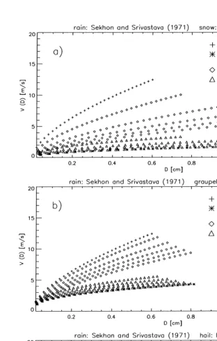
Obviously, the results depend on the employed fall speed parameterization. A review
Ž .
of fall speed parameterizations for rain and snow particles suggests that Eq. 4 gives the
Ž .
best results together with the parameterization of Sekhon and Srivastava 1971 for rain:
V D
Ž
.
s16.9 D0 .6Ž .
7Ž .
and the parameterization of Ferrier 1994 for snow, graupel, and hail: 0 .5
where r and r0 denote actual and surface air density, respectively.
Ž . Ž .
Fig. 1 shows an intercomparison of the formulae 4 and 5 for the above fallspeed
Ž . Ž . Ž .
parameterizations. Only Eq. 4 together with Eqs. 7 and 8 gives an almost
Ž .
continuous transfer between spectra. The use of Eq. 5 always causes a large discrep-ancy between almost melted and liquid spectra. In the case of other fall speed
Ž
parameterizations, discontinuities for both microphysical and optical properties e.g.
.
radar reflectivities are even stronger. Profiles from Doppler radar retrievals of fall speeds also indicate a steep increase of fallspeeds at FL right after the onset of melting with a rather smooth transition into the liquid rain layer below. In conclusion, the
Ž
insertion of melting layers under the above assumptions of flux constancy and
.
negligence of particle aggregation and break-up into prescribed hydrometeor profiles requires a continuous evolution of particle spectra during melting to avoid discontinuous profiles of microwave optical properties, e.g., radar reflectivity.
2.2.2. Water contents
Since the standard cloud model output provides only liquid water and ice contents above and below the FL, the water content available for melting has to be determined.
Ž .
Using the constant mass flux assumption in Eq. 3 and the definition of total flux integrated over the spectrum:
the amount of rain water resulting from melting a certain amount of ice can be
Ž .
calculated. With the definition of water mass above the FL e.g. for snow :
`
and by inserting N Dm into Eq. 10 using Eq. 3 , assuming constant particle mass:
D r1r3sD r1r3sD r1r3
Ž .
11procedure. Note that particle density was taken to be independent of diameter as prescribed by the cloud model.
Ž .
Let ‘i’ denote the layer index for which T zi )273.2 K and let ‘iq1’ be the layer
Ž .
index for which T ziq1 -273.2. If rain production in the stratiform portion of the cloud is considered to be from melting only, then the produced meltwater is:
MmŽr.sMr
Ž .
zi yMrŽ
ziq1.
Ž .
13The melted water from the frozen hydrometeors amounts to:
MmŽsqgqh.s
Ý
M zjŽ
iq1.
yMjŽ .
zi f ,j jss,g,hŽ .
14j
w Ž . Ž .x
If MmŽr.s MmŽsqgqh. thenÝ M zj iq1 yM zj i can be ingested as is by the melting model. Otherwise, it is assumed that no more water can be produced by the melting of frozen particles than is available from already melted water, i.e. MmŽr.. It follows that:
Mmsmin MmŽr., MmŽsqgqh.
Ž .
15Ž .
correcting M zr i afterwards to:
M)
Ž .
z sMŽ .
z yMŽ .
16r i r i m
This calculation ensures a conservative estimate of available meltwater, the conservation of water contents above and below FL as well as constant mass fluxes across the melting layer.
3. Mie-tables
Usually, radiative transfer routines use tables of the hydrometeor optical properties relevant to the passive microwave radiative transfer to enhance computational efficiency. These tables are computed after defining particle spectra and particle properties. Particle permittivity is a major uncertainty for melting particles. For problems of passive
Ž .
microwave radiometry, this has been recently investigated by Schols et al. 1999 , Fabry
Ž . Ž .
and Szyrmer 1999 or Meneghini and Liao 2000 . The main conclusion is that snow particles have to be treated differently than more dense particles such as graupel and
Ž
hail. According to results from various sensitivity studies Bauer et al., 1999, 2000;
. Ž .
Olson et al., 1999 , we employ a two-phase model for snow Fabry and Szyrmer, 1999 and the classical Maxwell–Garnett model with airrice inclusions in a host material composed of water for graupel and hail. Details can be found in the referenced literature. Approximations to microwave radiative transfer usually employ bulk hydrometeor
Ž
optical properties and do not require the calculation of an explicit phase function e.g.
.
Kummerow, 1993 . The input parameters, i.e., extinction coefficient be, single scatter-ing albedo vo, asymmetry parameter g, and backscattering coefficient bbs integrated over size spectra for each type, are given by:
`
p Qs cosu
2
with backscattering, scattering and extinction cross-sections Q , Q and Q , averagebs s e
Ž
scattering angle cosu at frequency n and temperature T which determine particle
.
permittivity , and liquidrice water content of rain, snow, graupel, hail, cloud water and
Ž .
cloud ice, qsqr,s,g,h,w,i which determine size spectra .
These parameters are integrated over hydrometeor types to obtain bulk cloud layer properties:
Our tables use indices for the independent variables which are: frequency, tempera-ture, hydrometeor type, and icerliquid water content, respectively. Thus, each parameter
Ž .
is a four-dimensional double-precision array of dimension 7, 6, 70, 500 as defined in Table 1.
The optical properties of melting particles are calculated only for snow and graupel. They are stored where Ts273 K, thus is70. For this, the melting layer is treated—as described in the previous sections—using the frozen water content of each species as input. The coarse vertical resolution of the cloud models requires an integration through the melting layer over small sublayers; thus, all melting stages:
zFL
where zFL denotes the altitude of the freezing level and h the depth of the melting layer. The increment is taken to be 20 m. At each level, z, the melting model calculates
meltwater fraction and corresponding mixed particle permittivity as well as all optical
Ž .
properties according to Eq. 19 , which are then stored in the Mie-tables. The tables contain the effective radar reflectivity, Z , instead of the backscattering coefficienteff calculated from:
1012l4
ny1
Zeffs<K <p5bbs, Krsnq2
Ž .
20r
where n denotes the complex refractive index and l the wavelength in centimeter. bbs is in units of cmy1.
Ž .
The scaling in Eq. 19 allows application to any layer depth, given that melting is completed within this layer. If the layer depth of the cloud model exceeds h, the optical properties can be calculated by adding the respective amount of liquid water left after melting over the remaining layer depth. As an output of these integrations, the total melting layer depth is also stored in the tables as the depth below FL at which all particles are completely melted.
A slight inaccuracy is introduced by the assumption that temperature is not constant throughout the melting process, as required by the melting model. The melting process produces latent cooling and may lead to almost isothermic conditions within the melting layer; however, this was assumed to be of minor importance.
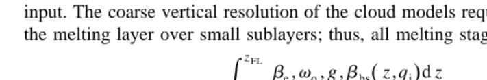
Fig. 2 shows an example of a cross-section through the stratiform part of a model cloud. The simulation was initialized over the Western Tropical Pacific on February 22,
Ž .
1993 and performed by the GCE model Tao and Simpson, 1993 on a 1-km resolution in the horizontal plane. The system represents a fast moving, bow shaped squall line almost parallel to the y-axis, which has developed a large stratiform tail at the time of
Ž . Ž y3. Ž .
this example ts210 min . The panels show the water contents in g m of rain a ,
Ž . Ž . Ž .
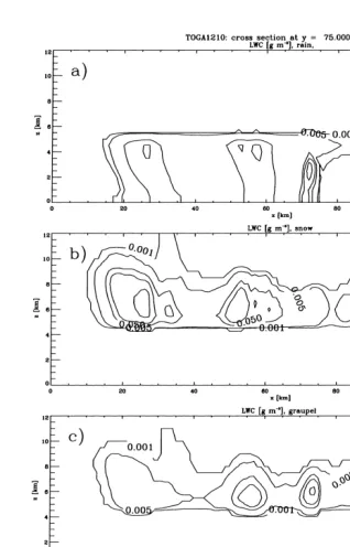
snow b , graupel c , and cloud liquid water d , indicating a well extended show and graupel layer on top of a rain layer. An area with low water contents was chosen to illustrate the melting model sensitivity. Fig. 3 shows the results for be and Zeff at 13.8 and 37.0 GHz for this cross-section after application of the described technique. A ‘bright band’ is visible for both parameters at zs5.5 km, indicating increased scattering and attenuation of radiation. In the melting layer, differences of 5–10 dBZ and doubling of be with respect to the liquid precipitation below are found, which correspond to observations that will be shown in the following section.
Since bright bands occur locally and only rarely cover areas of the size of the TMI footprints completely, the same GCE model simulation, but for a horizontal resolution of 3 km, was included for an assessment of primary resolution on net melting layer signature. From the same initialization, another model experiment was used to estimate the influence of different model parameterizations on the melting layer effect. For this purpose, four timesteps of the TOGA-COARE squall line simulation by the Meso-NH
Ž .
Ž . Ž .
Fig. 2. GCE model cloud cross-section at time step ts210 min. Water contents of rain a , snow b , graupel
Ž . Ž . y3
Ž . Ž . Ž
Fig. 3. Extinction coefficient a, c and effective reflectivity b, d for cross-section from Fig. 2 at 37.0 GHz a,
. Ž .
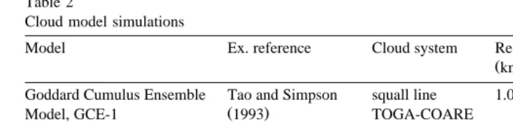
Table 2
Cloud model simulations
Ž .
Model Ex. reference Cloud system Resolution Time steps min
Žkm.
Goddard Cumulus Ensemble Tao and Simpson squall line 1.0 120, 150, 180, 210
Ž .
Model, GCE-1 1993 TOGA-COARE
Goddard Cumulus Ensemble Tao and Simpson squall line 3.0 180, 240, 300, 360
Ž .
Model, GCE-3 1993 TOGA-COARE
Ž .
Large Eddy Model CETPr Lafore et al. 1998 squall line 1.25 300, 360, 420, 480
Meteo-France, Meso-NH TOGA-COARE
and include cloud microphysics for five different particle types. For further information
Ž .
on mesoscale model intercomparison of this case, refer to Redelsperger et al. 2000 . Table 2 gives a summary of the employed model simulations.
4. TRMM observations
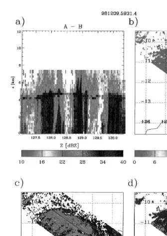
Fig. 4 presents an example of bright band occurrence in a storm system observed
Ž .
with the TRMM Precipitation Radar PR off the Northern coast of Australia. Spatial resolutions are ;4 km in the horizontal and 0.25 km in the vertical planes. Melting particles account for 5–10 dBZ increases of radar reflectivity as predicted by the model
Ž .
simulations Fig. 4a . The bright band is observed at altitudes between 4.0 and 4.5 km, according to the vertical velocity and temperature distributions. Fig. 4d indicates a high frequency of occurrence of bright bands compared to other rain types. However, due to the cross-track scanning illumination geometry of the PR, the bright band detection deteriorates towards the scan edges.
Ž .
A comparison of observed and simulated brightness temperature TB distributions was carried out to investigate the representativity of the described model approach. For the above introduced cloud model, four simulation time steps were chosen covering the mature and decaying stages of the squall line. The melting layer was introduced and
Ž .
radiative transfer simulations were carried out, applying the model of Bauer et al. 1998
Ž .
which includes the imaging specifications of the TRMM Microwave Imager TMI . TBs at 10.7, 19.35, 37.0, and 85.5 GHz and both polarizations were generated, assuming a
Ž
constant zenith angle of us52.88and varying azimuth angles. The first channel 10.7
.
GHz was simulated with an upgraded spatial resolution according to a deconvolution
Ž .
technique later applied to the TMI measurements Bauer and Bennartz, 1998 for the sake of an increased dynamic range of TBs.
Ž .
The standard output of the PR level 2 2A25 product provided by NASA was used in
Ž .
combination with TMI level 1 1B11 output. PR and TMI observations were colocated so that only PR observations were taken when they covered at least 80% of the TMI
Ž .
Ž . Ž .
Fig. 4. TRMM PR reflectivity vertical cross-section a , estimated rain rate at 2 km altitude b , altitude of
Ž . Ž .
bright band c , and rain system identifier d for tropical storm off the coast of Darwin, Australia, on December 9, 1998.
interesting rain cloud features represented in the measurements. The case from Fig. 2 was also included.
The effect of melting layers in observations and simulations was isolated as follows.
4.1. ObserÕations
Ž .
TBs were accepted if at least 80% of the TMI 10.7 GHz field of view FOV was covered with valid PR measurements and if at least 50% of the FOV was classified as rain-contaminated. Of these, observations were classified as stratiform, including a melting layer when the PR classification gave a minimum coverage by bright bands of
Ž .
50% sample size ns6916 . For stratiform clouds with no bright band, a maximum
Ž .
coverage by bright bands of 10% was permitted sample size ns2012 . This represents a compromise between discrimination of effects and large enough samples.
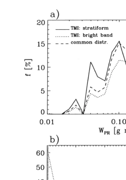
A very important aspect was the isolation of bright band effects from effects of systematic differences introduced into the samples from other sources: Fig. 5 shows histograms of near-surface rain liquid water contents, WPR, and remaining convective cloud fractions, C , from both datasets.c
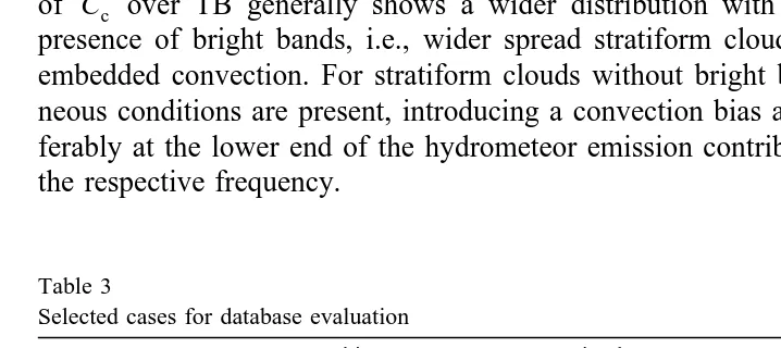
Those cases, including a bright band, contained slightly higher rainfall amounts and significantly less convection. To avoid biases in the following analysis, the original datasets were corrected by scaling with a common distribution obtained from the minimum frequency per liquid water and fractional convection interval. The distribution of C over TB generally shows a wider distribution with less total amounts in thec presence of bright bands, i.e., wider spread stratiform clouds with less occurrence of embedded convection. For stratiform clouds without bright bands, much less homoge-neous conditions are present, introducing a convection bias at narrow TB ranges—pre-ferably at the lower end of the hydrometeor emission contribution to the total signal at the respective frequency.
Table 3
Selected cases for database evaluation
Case Date Orbit no. System contained Lat.rion. of center
1 02r10r98 1171 tropical cyclone, Indian Ocean 158Sr608E 13–48 04r22r98– 2288– frontal systems with midlatitude origin
Fig. 5. Frequency distribution of near-surface rain liquid water contents from stratiform, bright band, and
Ž . Ž . Ž .
common observation datasets a . b As in a for fractional TMI EFOV coverage by convective clouds.
4.2. Simulations
TBs from the simulations were taken for which the root mean square difference between simulations including and excluding a melting layer over all frequencies exceeded 2 K. This was carried out for three different models but the same simulation experiment in order to investigate the impact of different model physics and resolutions
Ž
on the magnitude of the melting layer effect sample size ns2392, 6452, 1197 for
.
GCE-1, GCE-3, and Meso-NH, respectively .
Ž .
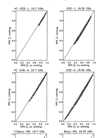
Fig. 6 compares the normalized polarization differences NPD of each profile for the melting vs. no melting case at 10.7, 19.35, and 85.5 GHz and all databases. NPD is defined as:
TB yTB
Ž
v h cloud.
NPDs
Ž .
21TB yTB
Ž . Ž . Ž .
Fig. 6. Simulated NPDs melting vs. no melting at 10.7, 19.35, and 37.0 GHz from GCE-1 a , GCE-3 b ,
Ž .
and Meso-NH c model experiments.
Ž .
decrease in transmittance, t, the offset to the line represents the decrease in t originating from the melting layer. All model simulations behave similarly with respect to the melting effect even though GCE-1 represents a less opaque situation. The decrease in t increases slightly with frequency as does the shielding of melting layer
Ž .
effects by the upper cloud layers, Bauer et al., 2000 so that the maximum effect is observed wheretf0.5 with Dtf0.05.
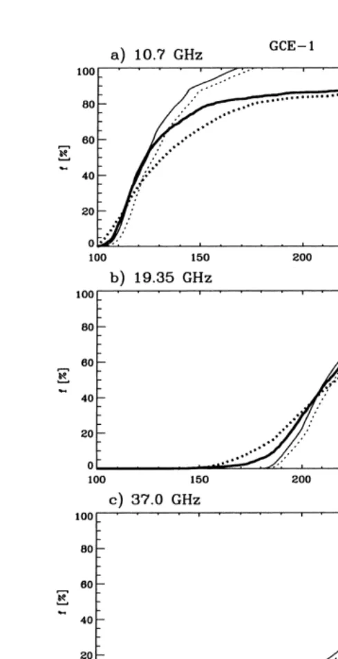
Since only from the simulations a profile-by-profile intercomparison is possible, accumulated distributions of TBs were compared to identify systematic differences between stratiform profiles containing significant amounts of melting particles and those without melting layer. The results between melting and no melting classes as well as observations and simulations are presented in Figs. 7–9. The thinrthick lines represent simulationsrobservations, respectively. One obvious difference between mo-del simulations and observations is the range of TBs and their distribution over this
Ž
range. While the model simulations always represent an isolated cloud system over a
.
certain time of its evolution , the observations cover a larger variety of system and cloud stages as well as surface conditions. This causes the observed TB-range to be wider with a more shallow slope compared to a more confined TB-variation in the simulations. The different models and resolutions already suggest that even when the same initialization was implemented, there is a strong dependence of TB-statistics on cloud model. The coarser GCE-3 produces stronger radiometric effects because the
Ž .
averaging over the TMI footprint size includes less grid cells see Fig. 8 . Thus, larger TBs occur at lower frequencies and lower TBs at higher frequencies. An obvious fea-ture in the Meso-NH simulation is the larger number of high TBs at 10.7 GHz and low TBs at 85.5 GHz, suggesting more precipitating water and ice than in the GCE simulations.
The melting layer effect is consistently represented in all simulations with amounts between 0 and 8 K over the whole TB range at lower frequencies. Theses values represent the shift in the TB-distributions, thus local differences can be much higher
ŽOlson et al., 1999 . At 85.5 GHz, the opacity of the cloud layers above the melting.
Ž .
layer reduces the TB-increase significantly Figs. 7d–9d . The TB-distributions from the observations compare very well with those from GCE-1 at frequencies above 10.7 GHz, keeping in mind the wider TB-range due to the larger variety of rain systems. Even at
Ž
85.5 GHz, where the strongest weakness of current cloud models i.e., the simula tion of
.
Ž .
Fig. 7. Accumulated frequency distributions of TBs from GCE-1 simulations thin lines and TRMM
Ž . Ž . Ž .
observations thick lines classified into stratiform solid lines and stratiform with melting layer dashed lines
Ž . Ž . Ž . Ž .
5. Summary and discussion
A method for the inclusion of melting layers in pre-calculated hydrometeor distribu-tions from bulk cloud models was presented, allowing a better representation in terms of radiometric and radar observations. A conservative approach was chosen to violate the model inherent microphysics as least as possible based on the assumption of constant mass flux through the melting layer. Particle microwave permittivity was treated
Ž .
differently for graupel and snow as described in Olson et al. 1999 . Tables of bulk optical properties at the frequencies of SSMrI and TMI were constructed for rain, snow, graupel, hail, cloud water and ice as functions of water content, temperature, and including the melting process.
Three cloud model experiments of the same initialization scenario were chosen, a melting layer was introduced, and radiative transfer simulations at the resolution of the TMI over an ocean surface were carried out. The relative shift of TB-distributions produced by melting particles ranged from 2 to 8 K at 10.7–37.0 GHz with negligible signatures at 85.5 GHz. Local differences, however, may be much higher. A consider-able set of colocated TMI and PR observations was produced. Based on the standard rain classification provided with the data, subsets of stratiform clouds and stratiform clouds with a radar bright band were constructed for an integral analysis of TB-dif-ferences among the sets. Unwanted effects such as biases by non-uniform rain intensity and embedded convection distributions were cancelled out. The bright band dataset showed similar TB-increases at low frequencies when compared to the simulations. At 85.5 GHz, the expected presence of larger particles in the observations with bright bands reversed the simulated TB-differences by increased scattering. This, however, is a not problem of the melting layer model but the result of the insufficient representation of particle spectra in current models.
The general picture seems to allow the identification of bright band effects from the chosen data classification approach; however, even the unification of rain and convec-tion distribuconvec-tions in both samples does not provide a clean profile-by-profile intercom-parison as was possible from the simulations. The sign and magnitude of the observed TB-changes introduced by the melting layer seem to confirm the simulations. The results also suggest that the presented model only provides a first order correction for bright band effects. In principle, the cloud model itself has to provide a more detailed treatment of the melting layer accounting for size spectra throughout the process. The introduction of a melting layer as described is somewhat disconnected from the cloud physics and cannot reproduce the occurrence of larger snow particles above the freezing level in widespread areas of descending mass. Thus, it represents a rather conservative model for the estimation of melting layer net radiometric effects.
Acknowledgements
Ž .
am grateful to Dr. W.S. Olson NASA GSFC for his valuable comments. This work
Ž .
was funded under contract 9122r97rNLrNB by the European Space Agency ESA .
References
Bauer, P., Bennartz, R., 1998. TMI imaging capabilities for the observation of rainclouds. Rad. Sci. 33, 335–349.
Bauer, P., Schanz, L., Roberti, L., 1998. Correction of three-dimensional effects for passive microwave remote sensing of convective clouds. J. Appl. Meteorol. 37, 1619–1632.
Bauer, P., Poiares Baptista, J.P.V., deIulis, M., 1999. The effect of the melting layer on the microwave emission of clouds over the ocean. J. Atmos. Sci. 56, 852–867.
Bauer, P., Khain, A., Pokrovsky, A., Meneghini, R., Kummerow, C., Marzano, F., Poieres Baptista, J.P.V., 2000. Combined cloud–microwave radiative transfer modeling of stratiform rainfall. J. Atmos. Sci. 57, 1082–1104.
Fabry, F., Szyrmer, W., 1999. Modeling of the melting layer. Part II: Electromagnetic. J. Atmos. Sci. 56, 3593–3600.
Ferrier, B.S., 1994. A double-moment multiple-phase four-class bulk ice scheme. Part I: Description. J. Atmos. Sci. 51, 249–280.
Kummerow, C.D., 1993. On the accuracy of the Eddington approximation for radiative transfer at microwave frequencies. J. Geophys. Res. 98, 2757–2765.
Lafore, J.P. et al., 1998. The Meso-NH atmospheric simulation system. Part I: Adiabatic formulation and control simulations. Ann. Geophys. 16, 90–109.
Meneghini, R., Liao, L., 2000. Effective dielectric constants of mixed-phase hydrometeors. J. Ocean. Atmos. Technol. 17, 628–640.
Mitra, S.K., Vohl, O., Ahr, M., Pruppacher, H.R., 1990. A wind tunnel and theoretical study of the melting behavior of atmospheric ice particles. IV: Experimental and theory for snow flakes. J. Atmos. Sci. 47, 584–591.
Mugnai, A., Smith, E., 1988. Radiative transfer to space through a precipitating cloud at multiple microwave frequencies. Part I: Model description. J. Appl. Meteorol. 27, 1055–1073.
Olson, W.S., Bauer, P., Viltard, N., Johnson, D.E., Tao, W.-K., 1999. A melting layer model for passiver ac-tive microwave remote sensing applications: Part I. Model formulation and comparison with observations. J. Appl. Meteorol. accepted.
Panegrossi, G. et al., 1998. Use of cloud model microphysics for passive microwave-based precipitation retrieval: significance of consistency between model and measurement manifolds. J. Atmos. Sci. 55, 1644–1673.
Redelsperger, J.L. et al., 2000. A GCSS model intercomparison for a tropical squall line observed during TOGA-COARE. Part I: Cloud-resolving models. Q. J. R. Meteorol. Soc. 126, 823–846.
Schols, J.L., Weinman, J.A., Alexander, G.D., Stewart, R.E., Angus, L.J., Lee, A.C.L., 1999. Microwave properties of frozen precipitation around a North Atlantic cyclone. J. Appl. Meteorol. 38, 29–43. Sekhon, R.S., Srivastava, R.C., 1971. Doppler radar observations of drop-size distributions in a thunderstorm.
J. Atmos. Sci. 28, 983–994.
Swann, H., 1998. Sensitivity to the representation of precipitating ice in CRM simulations of deep convection. Atmos. Res. 48, 415–435.