Adjustment procedures of a crop model to the site
specific characteristics of soil and crop using
remote sensing data assimilation
M. Guérif
∗, C.L. Duke
1Unité d’Agronomie I.N.R.A. de Laon Péronne, rue F. Christ, 02007 Laon Cedex, France
Received 14 July 1999; received in revised form 27 January 2000; accepted 14 February 2000
Abstract
Crop models can be useful tools for estimating crop growth status and yield on large spatial domains if their parameters and initial conditions values can be known for each point. By coupling a radiative transfer model with the crop model (through a canopy structure variable like LAI), it is possible to assimilate, for each point of the spatial domain, remote sensing variables (like reflectance in the visible and near-infrared, or their combination into a vegetation index), and to re-estimate for this point some of the parameters or initial conditions of the model. The spatial adjustment of the crop model provides, therefore, a better estimation of yield. This process has been tested on the re-estimation of crop stand establishment parameters and initial conditions for sugar beet (Beta vulgaris L.) crops, using the crop model SUCROS coupled to the radiative transfer model SAIL. The quality of recalibration depends in particular on the precision on the SAIL parameters other than LAI: soil reflectance, optical properties of leaves, and leaf angles. In applications on large domains, where these parameters may vary a lot, their estimation is an important factor in recalibration error. It was shown, using stochastic simulation, that beforehand knowledge of the variability of soil and crop characteristics considerably improved the results of the assimilation of reflectance measurements. The best results were obtained when the spectral reflectances were combined into the TSAVI vegetation index, which minimised the disruptive contribution of soil to the canopy reflectance. In particular, the use of TSAVI provided more consistent results for the estimates of the sowing date and emergence parameters, which remained poorer than yield estimates. Over a wide range of unknown crop situations corresponding to extreme sowing dates and emergence conditions, the proposed method allowed to estimate the sugar beet yield with relative errors varying from 0.6 to 2.6%. The results appeared to depend on the timing of remote sensing data acquisition; the best situation was when the data covered the whole period of LAI growth (including the highest values). © 2000 Published by Elsevier Science B.V.
Keywords: Local calibration; Reflectance; TSAVI; Error propagation; Stochastic simulation; Beta vulgaris L.
∗Corresponding author. Tel.:+33-3-23-23-64-88; fax:+33-3-23-79-36-15.
E-mail address: [email protected] (M. Gu´erif)
1Present address: Land Resource Research, Guelph University,
Guelph, Ont., Canada N1G 2W1.
1. Introduction
Crop models can be useful tools for estimating crop growth and yield on large spatial domains in order to monitor storage capacities, factories supply and or-ganisation. One of the greatest difficulties is that there is a need to know the value of parameters and/or initial 0167-8809/00/$ – see front matter © 2000 Published by Elsevier Science B.V.
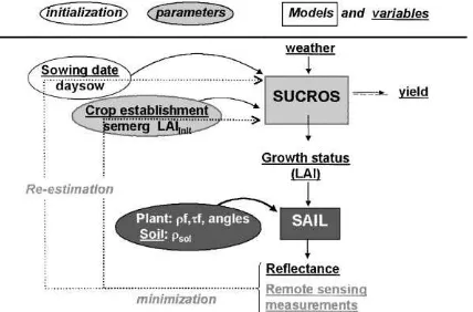
conditions for each field in order to apply the model to each point of the domain, and these may vary con-siderably from one point to another. This information is generally not available, but remote sensing, espe-cially in the optical domain, which gives extensive spatial information on the real crop growth status, is a practical way of estimating it. Several methods have been explored (Delécolle et al., 1992). One of them (Bouman and Goudriaan, 1990; Guérif and Duke, 1998) consists of coupling a radiative transfer model to the crop model (through a canopy structure variable like LAI), which makes it possible to simulate remote sensing variables (like reflectance in the visible and near-infrared) for each point of the spatial domain, at the times when remotely sensed reflectance data are available. Comparison of the simulated and measured variables allows re-estimation of some of the parame-ters or initial conditions of the model, leading to better simulation of yield. This process is called the assim-ilation of remote sensing data into the crop model; it provides a local adjustment of the crop model. Such a procedure was developed in a previous study on sugar beet (Guérif and Duke, 1998) that employed the SUCROS model (Spitters et al., 1989) and the SAIL model (Verhoef, 1984) for simulating radiative transfer into the canopy. The parameters describing the establishment of the crop (time between sowing and emergence, number of plants emerged, initial leaf area), which vary greatly according to soil, weather and sowing techniques were re-estimated for specific situations.
However, there is a need to know the value of the parameters of the radiative transfer model (other than LAI), which are specific to the status of canopies and soils (optical properties and geometry of the leaves, reflectance of the soil), and so vary greatly from place to place over a large domain. One should think about estimating them within the assimilation of remote sensing data technique also, but it would increase the number of parameters to be estimated and require a high amount of remote sensing data (which is hardly available in operational situations). It was shown that it is possible to develop a method for estimating the values of these parameters, based on prior analysis of their regional variations (Duke and Guérif, 1998). Using this method, instead of standard values, can re-duce the errors in spectral reflectance estimates made by the radiative transfer model.
The objective of this paper is to measure the in-fluence of these remaining errors (due to uncertainty of soil and canopy parameters) on the result of re-mote sensing data assimilation process, and hence on the estimates of crop model parameters, initial conditions and yield. The overall performance of the method was evaluated for estimating crop parameters and yield in virtual regional conditions where neither the initial condition (sowing date) nor some important crop parameters (crop establishment characteristics) are known. The study is restricted to sugar beet crops in northern France (Picardie). In the first part of the paper, the main statements of the previous mentioned studies are presented, then the methodology used and the results obtained in this work of error propagation analysis are presented and discussed.
2. The procedure used for crop model site specific adjustment
2.1. Variations in sowing dates, emergence and early growth characteristics
Farmers have tended to sow sugar beet earlier each spring during the past decade, in order to maximise the potential growth of the crop and the final root dry mass. These early sowing dates raised the probabil-ity of more difficult conditions during the sowing– emergence phase, leading to the appearance of mecha-nical obstacles for young plants (large soil aggregates due to soil humidity while drilling or crust formation due to rainfall after sowing). These difficult condi-tions may delay emergence (the temperature sum req-uired for emergence may rise from 100 to 180◦C day,
base 0◦C), decrease the proportion of plants which
can emerge (50% emergence rates compared to nor-mal rates of 95%), and therefore, result in fewer and smaller plants at emergence (Boiffin et al., 1992). These characteristics of crop establishment are key parameters of the SUCROS module for emergence and early growth, as they determine the initial LAI growth (Eq. (1)):
(deter-mined by the number of plants emerged and the initial leaf area per plant) and RGRL is the relative growth rate, which is quite stable whatever the crop establish-ment conditions (Boiffin et al., 1992). Both SEMERG and LAIinit may vary considerably (and be strongly intercorrelated) over a large spatial domain, depend-ing on the emergence conditions. Moreover, sowdepend-ing dates may also vary greatly according to soil traffica-bility and farmers decisions. This was confirmed by measurements that were made on two growing areas in Northern France in 1995 (Fig. 1). The time be-tween the earliest and latest sowing dates was about 6 weeks in both cases and the resulting emergence characteristics (thermal time from sowing to emer-gence and number of plants) varied as widely as that observed during experiments made on various sites and years (Boiffin et al., 1992). These variations have major effects on subsequent growth, as is shown by
Fig. 1. Frequency histograms (%) of sowing dates, thermal time from sowing to emergence (◦
C days, base 3◦
C) and number of plants emerged per m2 over 50 fields in two sugar factory areas;
(j): Eppeville and ( ): Marle (in 1995).
field experiments and by SUCROS sensitivity analysis (Guérif et al., 1998; Dürr et al., 1999). Thus, the real emergence parameter values are of major importance for simulation of subsequent growth: remote sensing is a powerful tool for estimating these parameters.
2.2. Crop model emergence and early growth module recalibration using assimilation of remote sensing data
The method was tested first on a local scale. SUCROS-sugar beet and SAIL models were coupled by means of the LAI variable (Fig. 2). Experimental data obtained for a ‘reference crop’, grown in poten-tial conditions, were used to calibrate the models in a previous phase, to adapt some of their coefficients to the regional context (Duke, 1997).
The method was tested on a different set of experi-mental data, for which crop establishment was inten-tionally disturbed. The default values for the parame-ters of emergence and early growth phases (SEMERG and LAIinit) were used in the SUCROS+SAIL model to simulate the spectral reflectance in three bands (green 500–590 nm; red 620–680 nm; near-infrared 790–890 nm), which was compared to four measure-ments made during crop establishment. Minimisation of a criterion based on the differences between sim-ulated and measured spectral reflectance using an optimisation software (FSEOPT) designed by Stol et al. (1992), enabled the method to re-estimate properly the emergence and early growth parameters as well
as the crop yield of the test crop (Guérif and Duke, 1998).
The initial condition (sowing date) and the SAIL model parameters of crop leaf angles and soil optical properties were known in this local scale application of the method. Transposition of this method to large spatial domains requires estimating such crop and soil parameters, which may vary considerably from one place to another. Furthermore, at this scale, sowing date is not available for each field and has to be esti-mated.
2.3. Variability of SAIL parameters on large spatial domains due to variations in soils and crops
2.3.1. Soil parameters
Soil spectral reflectance is an important parameter of the SAIL model. Its role is very strong during crop establishment until the canopy completely covers the soil surface. Soil spectral reflectance depends princi-pally on three soil characteristics:
1. Surface soil texture, which may be considered to be a permanent characteristic of soils. The infor-mation on soil texture spatial distribution is gen-erally available from soils maps: the predominant soil type in the region is a silty loam, with zones of clay loam and chalk classified as an Haplic Luvisol (FAO classification).
2. Surface humidity (0–1 mm), which changes quickly, depending on soil texture and the rain/ evaporation patterns (from 5 to 30% of soil dry mass). This information may be empirically de-rived from climatology (number of days since the last rainfall for a given evaporative regime) or from a crop model including a water balance module. 3. Surface rugosity, which depends mainly on soil
tillage operations and changes over time due to the action of the rain. Rugosity is low for seedbeds, but scuffling, which is done before canopy closure to eliminate weeds, may substantially increase it. Information on soil rugosity is quite difficult to ob-tain. Scuffling appeared to be applied to about 20% of the fields in the area.
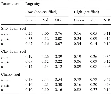
Field measurements on different soil types in the area, with varying humidity and rugosity, were used to derive parameters for soil spectral reflectance (ρsoil) as a decreasing exponential function of soil surface hu-midity (H, % dry mass)ρsoil=ρsmin+(ρsmin+(ρsmax−
Table 1
Parameters for exponentially decreasing soil reflectance–humidity functions for three main soil types and the two roughness classes Parameters Rugosity
Low (non-scuffled) High (scuffled) Green Red NIR Green Red NIR Silty loam soil rugosity (Table 1) (Duke and Guérif, 1998).
2.3.2. Plant reflectance parameters
The plant reflectance parameters in the SAIL model are the leaf optical properties (leaf spectral reflectance
ρL and transmittanceτL) and mean leaf angle (θL). Measurement of canopy properties to obtain a proper analysis of regional variations over a growing sea-son is extremely labour intensive. Thus, the results of a study done in 1994 on sugar beet crops expe-riencing various nitrogen regimes were used (Guérif et al., 1995). It was found (Guérif, unpublished results) that plant optical properties and structure parameters change with the crop’s age and the water and nitrogen regimes, which also affect LAI. The canopy proper-ties were expressed as a function of LAI in such a way that they are predictable using the growth model. Two periods were used to describe the canopy characteris-tics: emergence to LAI=2.0, and LAI>2.0. The means and standard deviations ofθL,ρLandτLare given in Table 2.
Table 2
Characteristics of sugar beet vegetation parameters for young and mature crops
LAI<2.0 LAI>2.0
Mean S.D. Mean S.D.
ρf Green 0.14 0.015 0.15 0.014
Red 0.06 0.007 0.07 0.008
NIR 0.46 0.001 0.46 0.001
τf Green 0.14 0.016 0.15 0.015
Red 0.05 0.011 0.06 0.071
NIR 0.49 0.001 0.49 0.001
θL 60.0 6.0 45.0 4.5
humidity was considered as dry (5%), intermediate (10%), or humid (25%). Therefore, the parameterisa-tions of soil reflectance–humidity relaparameterisa-tionships shown in Table 1 allowed the calculation of soil spectral re-flectance. Plant optical properties and geometry were derived from the mean values in Table 3, according to the estimate of LAI given by the model.
The errors in estimating canopy reflectance using both options were quantified by a Monte Carlo tech-nique (Duke and Guérif, 1998). Synthetic reflectance values (which represent an ‘image’ of the regional variations in crops reflectance and will be referred to hereafter as ‘real’ reflectance) were created with the SAIL model. The distributions given in Table 2 were used for the plant parameters. Uniform distributions of soil surface humidity within a class of humidity and the parameterisations of soil reflectance–humidity re-lationships in Table 1 were used for the soil parame-ters. For a given soil texture and a given class of sur-face humidity, series of 250 spectral reflectance (in the green, red and near-infrared bands) were simulated for a range of 10 LAI values from 0.05 to 6.0, by draw-ing parameter values from the distributions estimated from field measurements. The absolute errors on re-flectance estimate (E=ρreal−τsimulated) using options Table 3
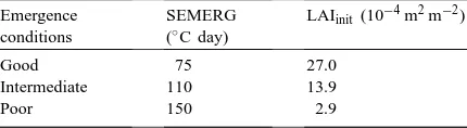
Parameters defining contrasted emergence conditions and crop establishment results
1 and 2 were computed for each situation and each spectral band.
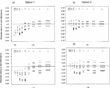
Option 2 allowed the estimation of SAIL parame-ters using prior knowledge of regional variability and this had many advantages over the standard estimates (Fig. 3). Option 1, with its standard values, overesti-mated reflectance for small values of LAI when soil reflectance has strong influence, while option 2 pro-vided estimates closer to the actual values.
The errors might be even larger for higher or lower soil surface humidity. When expressing the errors in terms of relative RMSE (Eq. (2)):
RRMSE= 250 for all the range of soil surface humidity, the errors appeared to be considerably reduced with our method of estimating SAIL parameters (Fig. 4), especially in the early part of the growing cycle (from 30 to 15%). The next major problem was to quantify the effects of the propagation of these errors due to variations in soils and crops on the results of the crop model recalibration using the assimilation of remote sensing data. This is the objective of the present work.
3. Method
A realistic scenario was simulated for estimating re-gional sugar beet yields using the crop model and the programming of five remote sensing data acquisitions during canopy establishment. The challenge was to assimilate the remote sensing data into the combined SUCROS+SAIL model and to re-estimate the sowing date (DAYSOW) and the emergence parameters (SE-MERG, LAIinit). A Monte Carlo type approach was also used.
3.1. Creation of virtual regional crop situations and associated reflectance
Fig. 3. Absolute errors in simulated reflectances for two spectral bands (red and near-infrared) on a silty loam of intermediate surface humidity: (a) red reflectance, option 1; (b) red reflectance, option 2; (c) nir reflectance, option 1 and (d) nir reflectance, option 2.
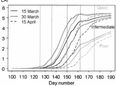
(rapid), intermediate, and poor (slow), characterised by three sets of (SEMERG, LAIinit) parameters (Guérif et al., 1998) (Table 3). SUCROS was run for the nine resulting combinations of sowing date and emergence parameters and for a given climatic year (1995), and provided a wide range of LAI time changes (Fig. 5). The differences in LAI between ex-treme situations reached as much as 4.4 (around Day 150) during canopy establishment.
The schedule for remote sensing data acquisitions consisted of five dates within this period, beginning 5 May (Day 125), ending 24 June (Day 175), with around 12 days intervals (cf. Fig. 5). For each of the nine crop situations and the five dates, virtual spectral reflectances were calculated, by running SAIL model. Each crop situation×date was characterised by a LAI value, given a soil type and a soil surface humidity class which allowed to draw the SAIL parameter values from the distributions of crop and soil
charac-teristics, as above. In that way, 250 temporal profiles of five spectral reflectances (in the green, red, and near-infrared bands) were calculated for each crop situation. A vegetation index, TSAVI, combining of red and near-infrared reflectance (Baret and Guyot, 1991), was also calculated using Eq. (3):
TSAVI= a(ρnir−aρr−b)
aρnir+ρr−ab+0.08(1+a2)
(3) where a and b are the coefficients of the soil line (ρsoil×nir=aρsoil×r+b), the subscripts ‘nir’ and and ‘r’ represent, respectively, the spectral reflectance in the near-infrared and the red bands.
3.2. Assimilation of the virtual reflectance to recalibrate the SUCROS+SAIL model
Fig. 4. Relative RMSE of simulated reflectances for the three spectral bands on a silty loam: (a) option 1 and (b) option 2. each of the nine crop situations, using the two ways of estimating SAIL parameters (options 1 and 2).
The criterion ‘crit’, which was minimised (Eq. (4)), was the root mean square difference between the spectral reflectance (three bands) simulated by the SUCROS+SAIL model and the ‘real’ spectral reflectance:
crit= 1
3×250 750
X
1
(ρreal−ρsimulated)2
!0.5
(4)
Constraints were imposed on the sowing date and emergence parameters estimated from this process of minimisation, so that they did not have ‘unreasonable’ values. As a result, 250 sets of (DAYSOW, SEMERG,
Fig. 5. LAI time changes for nine contrasted crop establishment situations, 1995. Time is expressed as the day number since 1 January. The vertical lines represent the dates at which remote sensing data are supposed to be available.
LAIinit) values were estimated. These new parameter values were then used to estimate LAI growth as well as the final yield.
The errors introduced in the estimate of spectral reflectance by estimating SAIL parameters, as well as the intrinsic error of the method, led to errors in the (DAYSOW, SEMERG, LAIinit) estimates. The errors concerning DAYSOW and SEMERG were quantified by RMSE. The errors concerning LAIinit, LAI and root dry mass were quantified by a relative RMSE (Eq. (5)):
RRMSE= 1
LAIinit×real
× 1
250 250
X
1
(LAIinit×real−LAIinit×simulated)2
!0.5
(5) For the nine crop situations, the ‘real’ values for DAYSOW were 15 and 30 March or 15 April, the ‘real’ values for SEMERG and LAIinit were those presented in Table 3. The ‘real’ LAI and root dry mass were those obtained by simulation with SUCROS model, using these sowing dates and emergence parameters.
4. Results
Fig. 6. Estimated root dry mass and simulated LAI time changes as resulting of the 250 processes of reflectance assimilation into SUCROS+SAIL model for a particuliar crop situation (medium sowing date, poor emergence, silty loam, intermediate soil surface humidity), and the two options for estimating SAIL parameters estimation. The solid line on LAI graphs represents the real LAI change with time, the dotted lines the simulated one. The vertical arrow on root dry mass graphs represents the ‘real’ value of yield. RRMSE values are reported.
date (30 March), with poor crop establishment con-ditions, assuming it was on a silty loam soil with an intermediate soil surface humidity, with the errors in reflectance estimates given in Fig. 3. The results ob-tained during the 250 processes of reflectance assim-ilation into the SUCROS+SAIL model are given in Figs. 6 and 7.
In order to compensate for the bad SAIL param-eter estimates by option 1 (cf. Fig. 3), which led to an over-estimation of reflectance (particularly in the near-infrared band), the assimilation process led to so-lutions that decreased ‘nir’ reflectance, and therefore, underestimated LAI (Fig. 6: most of the simulations are below the solid line which represents the real LAI change with time). Consequently, light interception, biomass production and root dry mass were underes-timated with option 1. In comparison, the use of more accurate estimates of SAIL parameters (option 2) in-stead of standard values (option 1), reduced greatly the errors in LAI and yield estimates: RRMSE dropped from 43 to 29% for LAI and from 7 to 4% for root dry mass, and there was no more bias.
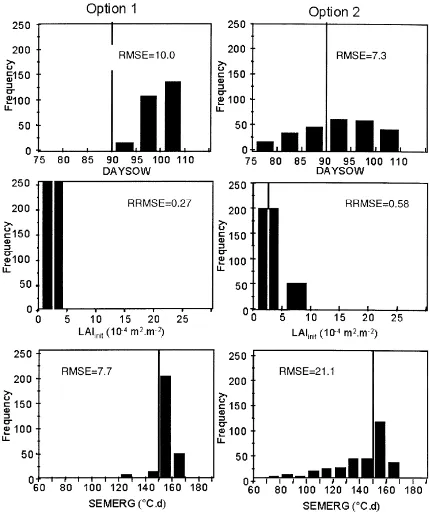
Fig. 7. Sowing dates and emergence parameters as resulting of the 250 processes of reflectance assimilation into SUCROS+SAIL model for a medium sowing date, poor emergence (soil condition: silty loam, intermediate surface humidity). The vertical arrow rep-resents the ‘real’ parameter value. RMSE (or RRMSE) values are reported. The abscissa extreme values are the constraints applied during the minimisation process.
Fig. 7 shows the associated estimates of sowing date and emergence parameters. With option 1, the tendency for the assimilation process to underestimate LAI was achieved by estimating very late sowing dates (estimated DAYSOW are always later than the real value). In comparison, the use of option 2 provided a better estimate of the sowing date (there is less bias and the RMSE is 3 days less than for option 1). The im-provement was not so clear for LAIinitand SEMERG, particularly because of compensatory effects between sowing date and these parameters on the response of the model (choosing a late sowing date is somewhat equivalent to choose a large SEMERG or to choose a little LAIinit).
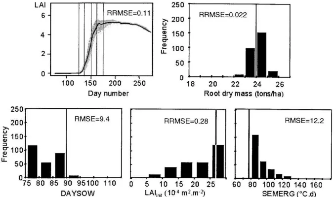
Fig. 8. LAI change with time, histograms of root dry mass, DAYSOW, SEMERG and LAIinit values as resulting of the 250 processes of
reflectance assimilation into SUCROS+SAIL model for a medium sowing date, good emergence crop situation (soil condition: silty loam, intermediate surface humidity), and option 2 for SAIL parameters estimation. The solid line on LAI graphs represents the real LAI change with time, the dotted lines the simulated one. The vertical arrows on the histograms represents the ‘real’ values. RMSE and RRMSE values are reported.
that the overall performances were better: RRMSE on LAI and root dry mass were significantly lower (2.2 and 10%) and the LAI growth curves were closed to the ‘real’ curve. This improvement in performance seemed to be linked to more appropriate remote sens-ing data acquisition dates, which provided complete cover of the fast growing period of LAI (see the ver-tical bars on the LAI graph on Fig. 8 and compare to the same features on Fig. 6). The estimates of sow-ing date and emergence parameters were not so good, again due to compensatory effects of these parameters in the minimisation process.
In summary, it appeared that the use of more ac-curate estimates of SAIL parameters obtained from a prior knowledge of regional variability instead of stan-dard values allowed better estimates of yield, which is the main objective. These results were even better when the timing of remote sensing data fit well the LAI growing period. More contrasted results were ob-tained on the retrieval of sowing dates and emergence parameters; they still needed to be improved.
Such an improvement could be achieved by using the vegetation index TSAVI to calculate the criterion to be minimised in the assimilation process, instead
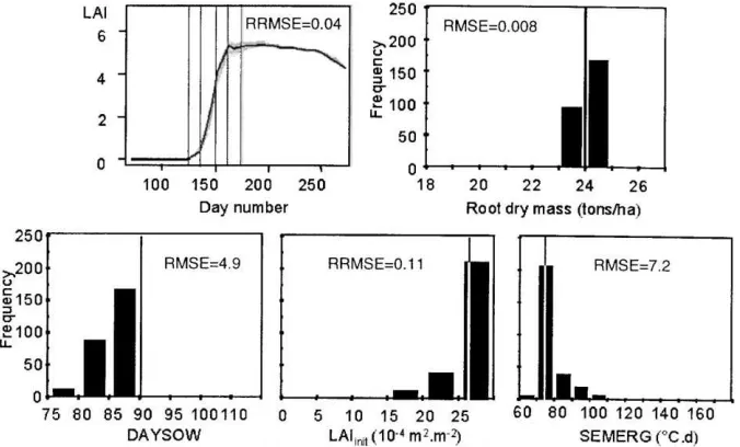
of using the spectral reflectance in the three bands; on the same type of crop situation (Fig. 9), the precision on sowing date and emergence parameters estimates was significantly improved (an RMSE of 4.9 days for sowing date, 7.2◦C days for SEMERG, which
corre-spond roughly to 1 day at this period of the year, and an RRMSE of 11% for LAIinit). At the same time, the errors on the root dry mass and LAI estimates were greatly reduced, reaching very low values (RRMSE of 0.8 and 4%). The improved ability of TSAVI to min-imise the contribution of soil reflectance to the canopy reflectance (Baret and Guyot, 1991) resulted in better performance of the crop model recalibration. Because of these interesting properties, TSAVI was therefore used as the best way of predicting both sowing and emergence parameters and crop growth variables and to compare the results for the whole range of crop situations.
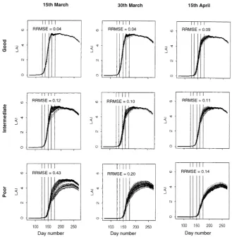
Fig. 9. LAI change with time, histograms of root dry mass, DAYSOW, SEMERG and LAIinitas resulting of the 250 processes of model
recalibration using TSAVI and option 2 for SAIL parameters estimation, for a medium sowing date, good emergence crop situation (soil condition: silty loam, intermediate surface humidity). The solid line on LAI graphs represents the real LAI change with time, the dotted lines the simulated one. The vertical arrows on the histograms represents the ‘real’ values. RMSE and RRMSE values are reported.
Compensatory effects among these parameters made it difficult to interpret correctly the ranges and sense of the errors.
The LAI dynamics simulated using the retrieved parameters (Fig. 10) confirmed that the results were
Table 4
Results of the 250 assimilation processes on the nine crop situations
Sowing date Emergence parameters Crop growth
RMSE RRMSE RRMSE
DAYSOW (day) SEMERG (◦
C day) LAIinit (%) LAI (%) RDMa(%)
15 March Gb 1.6 1.8 7.8 4.1 0.6
Ic 10.4 31.2 73.6 12.2 1.4
Pd 13.3 33.1 170.1 42.9 2.6
30 March Gb 4.9 7.2 11.1 3.5 0.8
Ic 3.1 9.6 30.2 10.2 1.0
Pd 3.9 9.9 64.6 20.0 1.6
15 April Gb 16.6 47.5 34.8 9.4 2.6
Ic 11.5 36.3 25.8 10.6 1.9
Pd 6.1 6.5 23.8 14.3 2.0
aRoot dry mass. bGood emergence. cIntermediate emergence. dPoor emergence.
Fig. 10. LAI changes with time as resulting of the 250 processes of reflectance assimilation into the SUCROS+SAIL model for the nine crop situations{emergence good, medium, poor}×{sowing date 15 and 30 March, 15 April}(soil condition: silty loam, intermediate surface humidity) using TSAVI, option 2 for SAIL parameters estimation. RRMSE values are reported.
on the graphs). The remote sensing dates are too early for the poor emergence results to give a correct fitting to the LAI curve and accurate estimates of the initial parameters; the simulated curves are widely scattered round the ‘real’ LAI curve (solid line).
The consequences on yield estimates at harvest are shown in Fig. 11: the relative RMSE of root dry mass ranged from 0.6% for early sowing and good emergence to 2.6% for poor emergence results or late sowing. The very high relative RMSE for LAI sim-ulations, had very little effects on yield estimate: the errors in high LAI have a major influence on the in-crease in the RRMSE of LAI, but these errors caused very little differences in light interception and hence
Fig. 11. Histograms of root dry mass estimates as resulting of the 250 processes of reflectance assimilation into SUCROS+SAIL model for the nine crop situations ({emergence good, medium, poor}×{sowing date 15 and 30 March, 15 April}) (soil condition: silty loam, intermediate surface humidity) using TSAVI, option 2 for SAIL parameters estimation. The vertical arrows on the histograms represents the ‘real’ values. RMSE and RRMSE values are reported.
5. Discussion
This study analysed the sensitivity of a crop model recalibration technique using remote sensing data assimilation to the variations in soils and crop char-acteristics that occur on large spatial domains. The main points of this study, carried on the coupled SUCROS+SAIL model, are that crop model recali-bration using canopy reflectance assimilation is quite effective for assessing yield. Better results were ob-tained with the use of more accurate estimates of SAIL parameters obtained from a prior knowledge of regional variability instead of standard values.
The best results were obtained when the spectral reflectance were combined into the TSAVI vegetation index, which minimised the disruptive contribution of soil to the canopy reflectance. In particular, the use of TSAVI provided more consistent results for the esti-mates of the sowing date and emergence parameters, which remained poorer than yield estimates. The main
reason for this poorer precision was the compensatory effects within these parameters on the response of the model, which provided more than one solution to the minimisation procedure.
The results appeared to depend on the timing of re-mote sensing data acquisition; the best situation was when the data covered the whole period of LAI growth (including the highest values). This may be due to smaller errors in the reflectance estimates for high LAI values and heavier weight in the definition of the crite-rion to be minimised. That aspect of timing of remote sensing data acquisition and the associated levels of precision will be hardly under control in operational conditions.
6. Conclusion
involved. The method may be applied in large-scale applications, like crop monitoring and yield predic-tion, or for precision agriculture, for adapting the cul-tural practices to within-field variability.
Great attention must be paid to additional weak-nesses and errors that inevitably accompany the ope-rational use of satellite or airborne remote sensing when planning any application of such a method. The number and the timing of available data may be highly speculative, and Moulin (1995) showed how such methods are sensitive to these things. Errors in the remotely sensed estimates of canopy reflectance, even after corrections for atmospheric effects, may also alter the performance of the method. Further studies are now necessary to investigate these aspects.
Acknowledgements
We thank Prof. J. Goudriaan and D. van Kraalingen for providing SUCROS and FSEOPT codes, and F. Baret for providing the SAIL code. This program was funded by the French Institut Technique de la Better-ave Industrielle and the French Programme National de Télédétection Spatiale.
References
Baret, F., Guyot, G., 1991. Potentials and limits of vegetation indices for LAI and APAR assessment. Remote Sens. Environ. 35, 161–173.
Boiffin, J., Dürr, C., Fleury, A., Marin-Laflèche, A., Maillet, I., 1992. Analysis of the variability of sugar beet (Beta vulgaris L) growth during the early stages. I. Influence of various conditions of crop establishment. Agronomie 12, 515–525.
Bouman, B.A.M., Goudriaan, J., 1990. Linking crop models and remote sensing data. In: Proceedings of the First Congress European Society of Agronomy, Paris, France, 5–7 December.
Delécolle, R., Maas, S.J., Guérif, M., Baret, F., 1992. Remote sensing and crop production models: present trends. ISPRS J. Photogramm. Remote Sens. 47, 145–161.
Duke, C., 1997. Assimilation de données de réflectance dans un modèle de fonctionnement de la betterave sucrière en vue de la prévision des rendements à l’échelle régionale. Doctoral Thesis, Institut National Agronomique Grignon, Paris, 141 pp. Duke, C., Guérif, M., 1998. Crop reflectance estimate errors from
the SAIL model due to spatial and temporal variability of canopy and soil characteristics. Remote Sens. Environ. 66, 286– 297.
Dürr, C., Guérif, M., Brochery, F., Ferré, F., 1999. Study of crop establishment effects on subsequent growth using a crop growth model (SUCROS). In: ESA International Symposium on Modelling Cropping Systems, Lleida, Spain, June 1999. Guérif, M., Duke, C., 1998. Calibration of the SUCROS emergence
and early growth module for sugarbeet using optical remote sensing data assimilation. Eur. J. Agron. 9, 127–136. Guérif, M., Machet, J.M., Droulin, J.F., 1995. Using remote sensing
to determine N status in the sugarbeet crop. In: Proceedings of the Symposium of the 58th Congress International Institute for Beet Research, Beaune, France, 19–22 June 1995, pp. 551–556. Guérif, M., Duke, C., Dürr, C., 1998. Spatial calibration of a crop model using optical remote sensing data. A case study on sugar beet emergence and early growth. In: Proceedings of the First International Conference on Geospatial Information in Agriculture and Forestry. Decision Support, Technology and Applications, Lake Buena Vista, FL, USA, 1–3 June 1998. ERIM International, Vol. 1, pp. 191–197.
Moulin, S., 1995. Assimilation d’observations satellitaires courtes longueurs d’onde dans un modèle de fonctionnement de culture. Doctoral Thesis, Université Paul Sabatier de Toulouse, 265 pp. Spitters, C.J.T., van Keulen, H., van Kraalingen, D.W.G., 1989. A simple and universal crop growth simulator: SUCROS87. In: Rabbinge, R., Ward, S.A., van Laar, H.H. (Eds.), Simulation and Systems Management in Crop Protection. Simulation Monographs 32, PUDOC, Wageningen, 434 pp.
Stol, W., Rouse, D.I., van Kraalingen, D.W.G., Klepper, O., 1992. FSEOPT a fortranprogram for calibration and uncertainty analysis of simulation models. Simulation Report CABO-TT, No. 24, CABO-DLO and Agricultural University, Wageningen, 24 pp.