*Corresponding author. Tel.:#1-506-453-4869; fax: #1-506-453-3561.
E-mail addresses: [email protected] (F.J. Arcelus); pablo@
upna.es (P. Arocena).
0925-5273/00/$ - see front matter (2000 Elsevier Science B.V. All rights reserved. PII: S 0 9 2 5 - 5 2 7 3 ( 9 9 ) 0 0 1 1 6 - 4
Convergence and productive e
$
ciency in fourteen OECD
countries: A non-parametric frontier approach
Francisco J. Arcelus
!,
*, Pablo Arocena
"
!Faculty of Administration, University of New Brunswick, P.O. Box 4400, Fredericton, N.B. E3B 5A3, Canada "Dpto. de Gestio&n de Empresas, Universidad Pu&blica de Navarra, Campus de Arrosadia s/n. 31006 Pamplona (Navarra) Spain
Received 29 December 1998; accepted 10 February 1999
Abstract
This paper explores the use of a non-parametric frontier approach to analyse multi-factor productivity across time and countries. We argue that conventional measures of total factor productivity involve some restrictive assumptions that might bias the results. A non-parametric approach avoids these assumptions. The model uses linear programming techniques to examine the productivity catching-up in 14 OECD countries over the 1970}1990 period, under the assumption of variable returns to scale. We"nd evidence of convergence, even if at quite di!erent speeds, for total industry, for manufacturing and for services. ( 2000 Elsevier Science B.V. All rights reserved.
Keywords: E$ciency; Productivity; Convergence; Data Envelopment Analysis
1. Introduction
Are less productive and developing countries catching-up to their more productive and de-veloped counterparts? Are less productive coun-tries growing faster than the most productive ones? To what extent there exists a common trend towards the convergence or divergence of produc-tivity levels among nations? These convergence queries are among the most salient and controver-sial issues in the economic growth "eld [1] and have been subject to a wide gamut of studies, of diverse objectives and methodology. Barro and
Sala-i-Martin [2], Quah [3], Sala-i-Martin [4], de la Fuente [5] and Durlauf and Quah [6] review this rather voluminous literature. It is the purpose of this paper to explore two important issues that still remain unresolved. We refer to the measure-ment of total factor productivity (heretofore, TFP) across time and countries and to the di$culty in disentangling the related e!ects of e$ciency, pro-ductivity and catching-up. For this purpose, the paper explores the use of a non-parametric frontier approach to analyse multi-factor productivity across time and countries. We argue that this ap-proach obviates the need for the rather restrictive assumptions inherent in the more traditional ap-proaches to the study of TFP comparability across time and countries.
appropriate indexes. Section 3 sets the stage for the estimation procedure by de"ning and contrasting the three concepts alluded to earlier, namely e$ -ciency, productivity and catching-up and by dis-cussing the issue of constructing productivity measures that di!erentiates scale from e$ciency e!ects, in the presence of variable returns to scale. Section 4 presents the basic methodology proposed in this study. It di!ers from the conventional ap-proach in that, following the pioneering work of FaKre et al. [7], we use a non-parametric method to construct a world frontier that serves as a bench-mark to compare the relative position of each country and its evolution over time. Section 5 presents the empirical results. We analyse the incidence of productivity catching-up across the 14 countries included in the OECD's International Sectoral Data Base [8]. The analysis is performed for the aggregated industry as well as for two sectors considered essential to the economic growth of any nation, namely manufacturing and services. Together, these two economic sectors rep-resent 77.5% of the total industry output in 1970 and 84% in 1990 for the countries included in the ISDB data base. We"nd evidence of a high degree of convergence for all three sectors and provide reasons for any discrepancies with past studies on the subject. A Conclusions section completes the paper.
2. The problem of measuring total factor productivity
This section considers the two basic problems associated with the measurement of TFP, namely (i) lack of readily available and generally accept-able data on both labour and capital inputs, as well as lack of widely accepted conversion factors for output; and (ii) the restrictive assumptions re-quired to measure TFP levels for any inputs-to-output conversion approach.
The"rst issue is re#ected in the literature
prim-arily through the use of partial productivity indices as the basic measurement index of convergence, normally proxied by GDP per capita or similar income variable. Typical studies of this type are the pioneering works of Baumol [9] and Abramovitz
[10] which provide evidence of technological catching-up between industrialised countries espe-cially during the post-war period. Other examples include those of Barro and Sala-i-Martin [11,12] and Sala-i-Martin [4,13]. These studies show evid-ence of convergevid-ence across countries and regions
by "nding a signi"cant inverse relationship
be-tween the GDP growth and a country's initial level of productivity in a cross-section regression. In contrast, Quah [4,13,14] "nd support for club convergence or polarisation of economies into groups of rich and poor. Barro and Sala-i-Martin [2] and Durlauf and Quah [6] survey this literature.
A drawback of this literature is that a partial productivity index improvement might be ex-plained by an input substitution process and not by an e$ciency improvement in the input usage. An important implication of this observation is the advisability of measuring the combined e!ects of all productivity factors, hence the need for TFP indi-ces. Examples include Dowrick and Nguyen [15], Bernard and Jones [16], Cronwell and WaKchter [17] and FaKre et al. [7], among others. Dowrick and Nguyen [15]"nd strong evidence of TFP con-vergence for 14 OECD countries between 1950 and 1985, using capital and labour growth rates as well as the initial relative level of per capita GDP as independent variables to explain the growth of GDP. Bernard and Jones [16] also use TFP indices to compare the productivity performance, across several sectors, of the same 14 OECD countries used in the present study, for the 1970}1987 time period. Its principal "ndings are evidence of con-vergence if at di!erent speeds among most sectors of the economy. The service sector exhibited the highest speed of convergence or catching-up, with poor to non-existent convergence results for manu-facturing. Therefore, services are mainly explaining the catching-up process detected for the total industry.
an underlying production function that character-ises the existent technology, such as the Cobb} Douglas production function; (ii) constant returns to scale; (iii) an optimising behaviour, with no room for any ine$ciency, be it technical or al-locative; and (iv) the use of a Hicks neutral tech-nical change to calculate the TFP growth. The limiting aspects of these assumptions are re#ected in the construction of the most popular TFP index, the Tornqvist index. Based upon a discrete approx-imation of the general Solow [19] model, it requires cost shares as weights and assumes these shares to be cost-minimising shares (i.e. factor pri-ces are equal to their value marginal products). However, as Bernard and Jones [16] point out,
`depending on the relative price used to weight apples and oranges, either country may appear to be more productive than the othera (p. 1232). Hence, the computation of TFP levels requires assumptions that are di$cult to justify in practice. Whenever these assumptions do not hold, TFP measurements will be biased.
Although its focus is not on the productivity convergence per se, FaKre et al. [7] analyse TFP growth in 17 OECD countries over the period 1979}1988 through the computation of the Malm-quist productivity index. Recent surveys on the Malmquist index appear in Coelli et al. [18] and FaKre et al. [20]. Such an alternate approach to traditional productivity measurement does not require the four assumptions outlined earlier and thus avoids the corresponding measurements pit-falls outlined in this section.
3. E7ciency,productivity,scale and catching-up
With respect to the concept of convergence, there are two issues of importance, namely (i) the exact meaning of the term `convergencea; and (ii) the standard against which each country is measured. Convergence may be broadly de"ned as the tend-ency for two or more economies to become more similar, be they in terms of per capita incomes, or in#ation rates, or growth rates or such similar measure. Barro and Sala-i-Martin [2,11,12] and Sala-i-Martin [4,13] identify two types of conver-gence b-convergence and p-convergence. On the
one hand, there exists b-convergence in a cross-section of economies, if poor economies tend to grow faster than wealthy ones. That is, productivity convergence may be de"ned as catch-up by low-productivity economies to higher low-productivity ones. On the other hand, a group of economies exhibits p-convergence if the dispersion of their productivities tend to decrease over time. Estimates of both types of convergence are presented in Section 5. It should be observed that only uncondi-tional, also denoted absolute,b-convergence is con-sidered in this paper, following the lead of most papers using OECD data (e.g. [4,16,17]). The rationale for this approach lies on the relative homogeneity of the OECD countries, at least as compared to the rest of the countries of the world [2,4], which leads towards ignoring the additional socio-economic variables usually included to derive measures of conditional b-convergence. Durlauf and Quah [6] provide a compilation of the wide range of variables used in the empirical studies of conditional b-convergence. Further, Durlauf and Quah [6] and De la Fuente [5] summarise various conceptual and estimation aspects associated with the nature and use of
b-convergence.
As for the second issue, convergence "rstly re-quires the identi"cation of the most productive countries in order to construct a behavioural refer-ence or a benchmark for the rest of the economies. The distance that separates it from that benchmark explains the relative performance of one country. If that distance becomes smaller over time we will say that there is convergence. This is in contrast to the traditional approach of measuring TFP growth for one economy exclusively on the basis of the country's past performance.
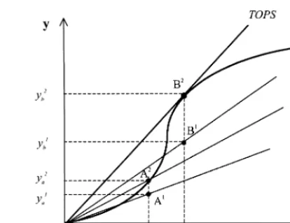
Fig. 1. The productive e$ciency under variable returns to scale.
Fig. 2. Catching-up under variable returns to scale.
standard or norm [22]. In this respect, e$ciency ranks the productivity of two or more units [23]. Fig. 1 illustrates this fact in a single input}output situation, where the production technology is rep-resented through the curveF(y,x), that de"nes the maximum output attainable from each level of input. All input}output combinations below this curve are feasible but technically ine$cient. Thus, economic unit B producesy1b withx1b in period 1, but it could obtainyH
b"hy1b, whereh"yHb/y1b(*1) is the Farrell's (1957) output measure of technical ine$ciency. In contrast, the same unit in period 2 (B2) is e$cient since it produces the maximum output attainable, given the existing technology. That is, production is occurring on the boundary of the production possibilities set, therefore
y2H
b /y2b"1. However, both observations exhibit the same average productivity (y/x) measured by the slope of the ray 0B.
In the simplest case of one input (i.e. labour) and one output (i.e. GDP) under constant returns to scale, it is obvious that the catching-up re#ects the productivity change. The most productive country presents the highest ratio of average productivity and it constitutes the reference for the rest. If the other countries increase their average productivity ratio more than the leader, they are considered to be`catching-upato it. However, this is not neces-sarily true under variable returns to scale, even in the simplest of cases, namely that of one input and one output. To illustrate this point, consider Fig. 1,
where the technology of production exhibits vari-able returns to scale, with the optimal scale given by the maximum average productivity at pointS. Observations on the left ofSare too small and are operating in the region of increasing returns to scale. On the other hand, observations on the right ofSare too large and are operating in the region of decreasing returns to scale. Now consider two economies, A and B, in two periods, with no tech-nical change between them (any shift in the produc-tion frontier). In our example, B is more productive than A in both periods, as shown by the higher slope of the ray 0B. Let us assume than in period 2, B moves to B
2 and A to A2. This move implies a change in the scale of operations and the elimina-tion of technical ine$ciency, but the average pro-ductivity remains unchanged. Both economies are now technically e$cient, although they are still operating far from the optimal scale. Although these moves reveal an obvious catching-up to the frontier we would conclude that no convergence across economies has occurred: the cross-sectional variance remains constant (nop-convergence) and the rate of growth (zero) is equal for both countries (nob-convergence).
economiesin the sense ofb. As a result, the conven-tional cross-section regression analysis would show a positive correlation between productivity growth and the initial productive level. Fig. 2 illustrates the consequences of ignoring the existence of scale economies in measuring productivity change. Imposing constant returns to scale implies assum-ing that the maximum average productivity is at-tainable for any country, irrespective of its scale size. Hence, we compute changes in the distance from each observation to the maximal productivity showed at the technically optimal scale. This leads to the rayTOPSin Fig. 2, which includes all combi-nations having the same (maximal) average produc-tivity as theS point in Fig. 1 and constitutes the constant returns to scale frontier. As F+rsund [23] remarks, since we are analysing the variable returns to scale technology de"ned byF(y,x) these combi-nations (apart from S) are not feasible; they just serve as points of comparison. However, when vari-able returns to scale are taken into account in the construction of the benchmark, the conclusion is fairly di!erent: both countries are located at the best practice frontier in period 2.
The main import of the above discussion is that the actual productivity change may not re#ect the relative catching-up, because of the in#uence of the returns to scale of the frontier technology. The more signi"cant the scale e!ects are, the higher the discrepancy will be, since moving closer to TOPS may require changes both in e$ciency and scale. Furthermore, if di!erences in scale persist through-out the time, the assumption of constant returns to scale leads to increases in the probability of detect-ing divergence, even though all economies are clos-ing the distance that separates them from the best practice benchmark. For this reason, we consider the notion of productive e$ciency to be more appropriate than that of productivity, for the pur-pose of analysing convergence as catching-up, in the presence of variable returns to scale.
4. A non-parametric frontier model
We analyse productive e$ciency through non-parametric frontiers or data envelopment analysis (DEA). Charnes et al. [24], Lovell [25] and Cooper
et al. [26] provide a comprehensive survey on DEA methodology and applications. A DEA model con-structs a best practice frontier from the observed inputs and outputs as a piecewise linear techno-logy. The frontier technology is formed as linear combinations of observed extremal activities (best practice), yielding a frontier consisting of facets. This technology can be shown to satisfy very gen-eral axioms of production theory (see [27]). (In)e$ciency is measured by the distance of each observation to that frontier. DEA is typically applied to cross-section data to assess productive e$ciency of one economic unit for a particular time period.
Although there exist a considerable amount of DEA literature, the utilisation of panel data in empirical applications of DEA is still limited. Charnes et al. [28] introduced the so-called` win-dow analysisa, for measuring changes of perfor-mance over time. A di!erent approach to the measurement of e$ciency and technical change between two periods of time was developed by FaKre et al. [29], through the use of DEA to construct the Malmquist index [30] of productivity change. We integrate the time into e$ciency assessment in a dif-ferent way. Our panel data includesJcountries and ¹years. Using all the data, i.e., the¹]J observa-tions, we construct a reference frontier or what Tulkens and Vanden Eeckaut [31] call an` inter-temporal frontiera. This is equivalent to consider-ing a country in each di!erent year as if it were a di!erent observation in a cross-section analysis. As a result, it is possible to compare each observa-tion to the rest countries and to their own past performances, by computing the extent to which less productive countries move closer to the best practice frontier, as de"ned by the most productive countries throughout the whole observation period. In this way, we have a stable reference in relation to which we measure the productive e$ -ciency level achieved by each country from
t"1,2,¹. Then, if one country improves its
rela-tive position over time in relation to the rest, it will reduce the distance to the frontier. In other words, it will catch-up to the most productive countries that form the best practice frontier.
the frontier. This function is the reciprocal of the Farrell's [33] output measure of technical e$ cien-cy, which is in turn equal to the maximal propor-tional expansion of the output vector y, given inputsx. Following FaKre et al. [27], a production technology transforming inputs x3RN
` into out-putsy3RM
`can be represented by theGraphof the technology, i.e. by the set of all feasible input} out-put vectors, as follows:
GR"M(x,y):xcan produceyN.
The output distance function is de"ned by
D
0(x,y)"minMh: (x,y/h)3GRN
"[maxMh: (x,hy)3GRN]~1.
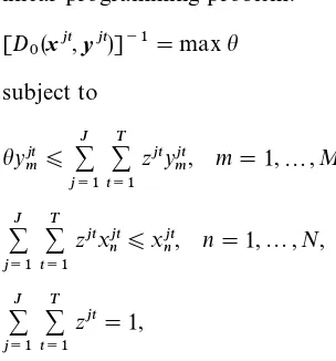
We consider a reference technology which allows variable returns to scale and satis"es strong dis-posability of inputs and outputs (see FaKre et al. [34] for details). Under these assumptions, the distance function can be computed by solving the following linear programming problem: tion i is on the frontier, because it achieves the maximum output obtainable from any country of the reference set, given its level of inputs. On the contrary, ifD
0(xi,yi)(1 (hi'1), observationiis not e$cient, because there exists some unit or a convex combination of other referent units located on the e$cient frontier, that utilises the same quantity of inputs and produce a higher level of outputs. For each sector, we solve the above
problem ¹]J times, one for each observation (xjt,yjt), withj representing the country andt the year in our case.
5. Data and results
The data are drawn from the 1996 version of the International Sectoral Data Base [8], compiled by the OECD as part of its on-going project to study the industrial structure and economic performance of its members. The current version includes information for 14 countries (Austria, Belgium, Canada, Denmark, Finland, France, Germany, Great Britain, Italy, Japan, Netherlands, Norway, Sweden and USA). The ISDB [8] covers the 1960}1995 time period. However, the gaps for the pre-1970 and the post-1990 years were considered to be signi"cant enough to drop these years from consideration. As a result, the paper uses data drawn for 1970}1990 time period, for which there are no gaps, with the exception of the Netherlands and the last two years of Finland for the service sector, and the last year for Great Britain in the total industry case.
The proxies for labour and capital are the num-ber of employees, and the gross capital stock (US dollars at 1990 prices, and 1990 PPPs). The output is measured by the GDP (US dollars at 1990 prices, and 1990 PPPs). Total Industry and Manufactur-ing correspond to the ISDB codes TIN and MAN respectively. Services include the ISDB codes RET (wholesale and retail trade, restaurants and hotels), TRS (transport, storage and communication), FNI
("nance, insurance, real state and business services)
and SOC (community, social and personal servi-ces). Total Industry includes agriculture; mining and quarrying; electricity, gas and water; manufac-turing; services and construction. Further details on an earlier but still valid ISDB version appears in Meyer-zu-Schlochtern and Meyer-zu-Schlochtern [35]. For each country and sector, the results are presented in summary form for the 1970}1975, 1975}1980, 1980}1985 and 1985}1990 time periods in order to distinguish possible di!erent patterns of performance in each period.
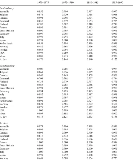
Table 1
The impact of variable returns to scale
1970}1975 1975}1980 1980}1985 1985}1990 Total
Total industry
Australia 0.952 0.986 0.997 0.997 0.982
Belgium 0.874 0.930 0.958 0.988 0.934
Canada 0.994 0.998 0.994 0.992 0.994
Denmark 0.655 0.679 0.653 0.735 0.679
Finland 0.585 0.682 0.718 0.710 0.669
France 0.996 0.991 0.993 0.990 0.993
Great Britain 0.990 0.995 0.997 0.996 0.994
Germany 0.997 0.995 0.992 0.989 0.993
Italy 0.997 0.993 0.992 0.998 0.995
Japan 0.999 1.000 1.000 1.000 1.000
Netherlands 0.951 0.984 0.999 0.998 0.981
Norway 0.482 0.568 0.596 0.652 0.570
Sweden 0.963 0.994 0.978 0.959 0.973
USA 0.993 0.989 0.986 0.982 0.988
Mean 0.888 0.913 0.918 0.928 0.910
St. dev. 0.170 0.144 0.140 0.122 0.145
Manufacturing
Australia 0.906 0.905 0.924 0.934 0.917
Belgium 0.869 0.856 0.869 0.906 0.875
Canada 0.940 0.943 0.959 0.966 0.951
Denmark 0.708 0.702 0.707 0.744 0.715
Finland 0.735 0.779 0.797 0.775 0.770
France 0.983 0.985 0.986 0.986 0.985
Great Britain 0.991 0.990 0.989 0.989 0.990
Germany 0.994 0.993 0.993 0.994 0.993
Italy 0.982 0.985 0.987 0.991 0.986
Japan 0.999 0.997 0.997 0.998 0.998
Netherlands 0.891 0.903 0.927 0.958 0.918
Norway 0.621 0.585 0.522 0.504 0.561
Sweden 0.878 0.877 0.872 0.887 0.878
USA 1.000 0.989 0.998 1.000 0.997
Mean 0.893 0.892 0.895 0.902 0.895
St. dev. 0.118 0.121 0.133 0.136 0.127
Services
Australia 0.979 0.996 0.998 0.999 0.992
Belgium 0.991 0.995 0.978 1.000 0.991
Canada 0.998 0.999 0.999 0.999 0.999
Denmark 0.618 0.632 0.618 0.688 0.638
Finland 0.537 0.556 0.606 0.638 0.576
France 1.000 1.000 1.000 0.994 0.998
Great Britain 0.994 0.999 0.999 1.000 0.998
Germany 0.999 0.999 1.000 0.995 0.998
Italy 1.000 1.000 1.000 1.000 1.000
Japan 0.999 0.992 0.988 0.993 0.993
Norway 0.448 0.588 0.654 0.725 0.597
Sweden 0.964 0.935 0.879 0.894 0.920
USA 1.000 1.000 0.998 0.996 0.998
Mean 0.887 0.899 0.901 0.917 0.900
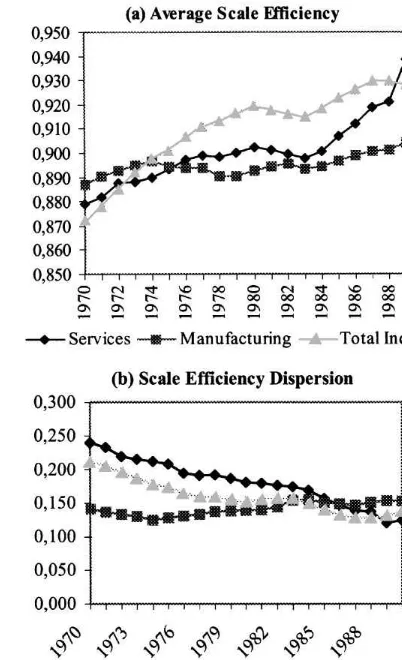
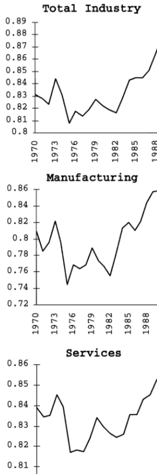
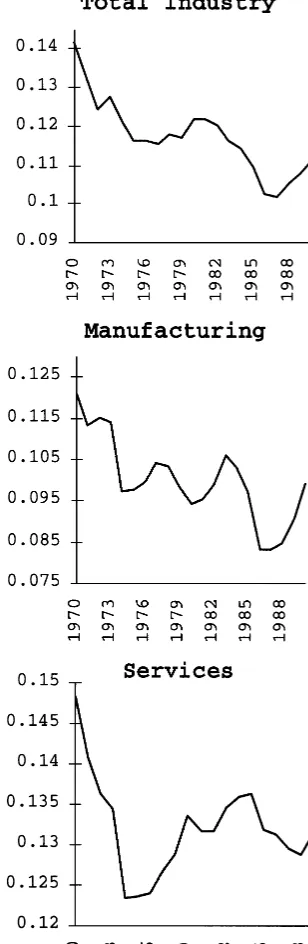
Fig. 3. The evolution of the average scale e$ciency and its dispersion.
exhibited by the various sectors, for the various countries and time periods. For each sector/year/ country combination the linear program of (1) was run twice, with and without the equality con-straint, to obtain the distances of each unit to the frontier (variable returns to scale allowed) and to the optimal scale on the frontier function (calculated for a constant returns to scale fron-tier), respectively. The presence of constant (vari-able) returns is detected when the ratio of the second to the "rst index for a particular sector/ year/country combination equals (is less than) one [36]. If there are not scale e!ects, then all observa-tions should be equally technically e$cient, relative both to variable and constant returns to scale fron-tier. On the other hand, departures from the opti-mal scale will be re#ected in scale e$ciency ratios under one.
Even a cursory look at Table 1 suggests the presence of variable returns for most cases. For total industry, only Japan is operating at the opti-mal scale for the entire period under study. The rest of countries display scale ratios lower than unity, re#ecting various degrees of scale economies. In the manufacturing sector, seven countries (Norway, Denmark, Finland, Belgium, Sweden, Australia and The Netherlands) present very low average values, as a consequence of operating far from the optimal scale throughout the whole period. Only Japan (in 1970}1972) and the US (for the whole period with the exception of 1978}1981) appear as scale e$cient. In services, Italy, France, the US and Japan are scale e$cient most of the time and Belgium, only in the last two years. At the other end, the Scandinavian countries appear very scale ine$cient in comparison with the rest. Fig. 3 dis-plays the evolution of the average scale e$ciency and its dispersion by sector. Panel (a) shows that total industry and the services sector exhibit a
sig-ni"cant increase in scale e$ciency, i.e. countries are
on average moving closer to the optimal scale. By contrast, only the last seven years of the period show a moderate increase in the average scale e$ -ciency for the manufacturing sector. Panel (b) dis-plays the dispersion on the scale e$ciency in the form of the coe$cients of variation (see also the last row of Table 1). Whereas pronounced decreases in dispersion are detected in total industry and
services, the disparities remain for the manufactur-ing sector throughout the period, even becommanufactur-ing wider during the 1980s. This evidence suggests the need to evaluate convergence under variable re-turns to scale.
Table 2
Average e$ciency scores
1970}1975 1975}1980 1980}1985 1985}1990 Total
Total industry
Australia 0.812 0.812 0.816 0.837 0.819
Belgium 0.991 0.975 0.988 0.993 0.987
Canada 0.738 0.758 0.740 0.768 0.750
Denmark 0.859 0.844 0.905 0.848 0.864
Finland 0.903 0.756 0.763 0.844 0.821
France 0.724 0.768 0.782 0.831 0.774
Great Britain 0.663 0.653 0.683 0.782 0.694
Germany 0.739 0.780 0.774 0.814 0.775
Italy 0.839 0.913 0.935 0.982 0.914
Japan 0.949 0.933 0.947 0.980 0.952
Netherlands 0.853 0.879 0.870 0.900 0.874
Norway 0.985 0.894 0.903 0.924 0.929
Sweden 0.561 0.545 0.563 0.604 0.568
USA 0.969 0.964 0.950 0.993 0.969
Mean 0.827 0.820 0.830 0.864 0.835
St. dev. 0.127 0.118 0.116 0.106 0.117
Minimum 0.561 0.545 0.543 0.604 0.568
Manufacturing
Australia 0.766 0.776 0.759 0.804 0.776
Belgium 0.787 0.826 0.945 0.986 0.881
Canada 0.787 0.797 0.739 0.784 0.777
Denmark 0.872 0.830 0.861 0.775 0.836
Finland 0.631 0.587 0.660 0.796 0.667
France 0.819 0.817 0.817 0.830 0.821
Great Britain 0.708 0.625 0.591 0.704 0.659
Germany 0.883 0.865 0.837 0.876 0.866
Italy 0.604 0.710 0.760 0.869 0.730
Japan 0.897 0.804 0.828 0.885 0.855
Netherlands 0.692 0.722 0.738 0.766 0.728
Norway 0.981 0.874 0.929 0.950 0.936
Sweden 0.735 0.654 0.686 0.732 0.703
USA 0.925 0.936 0.874 0.975 0.928
Mean 0.792 0.773 0.787 0.838 0.797
St. dev. 0.110 0.100 0.100 0.088 0.100
Minimum 0.601 0.572 0.591 0.699 0.615
Services
Australia 0.841 0.841 0.864 0.865 0.852
Belgium 0.994 0.971 0.981 0.984 0.983
Canada 0.750 0.730 0.727 0.755 0.741
Denmark 0.969 0.966 0.986 0.941 0.966
Finland 0.955 0.905 0.855 0.866 0.901
France 0.720 0.744 0.751 0.805 0.753
Great Britain 0.747 0.742 0.761 0.839 0.771
Germany 0.707 0.733 0.739 0.797 0.742
Italy 0.878 0.943 0.955 0.984 0.937
Japan 0.981 0.939 0.965 0.994 0.970
Netherlands * * * * *
Norway 0.854 0.690 0.631 0.626 0.708
Sweden 0.528 0.557 0.590 0.605 0.568
USA 0.934 0.960 0.979 0.998 0.966
Mean 0.835 0.825 0.830 0.851 0.835
St. dev. 0.134 0.129 0.134 0.130 0.132
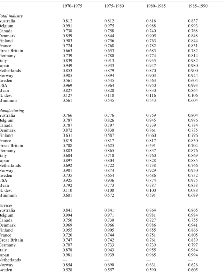
Fig. 4. The evolution of average productive e$ciency scores by sector.
two sectors, the variability in the rates of increase suggests substantial potential for further produc-tive e$ciency improvements in many countries.
The dispersion of the scores in the form of stan-dard deviation is displayed at the bottom of Table 2. The dispersion data indicate that, for total industry and manufacturing, higher e$ciency levels are also accompanied by reductions in the variabil-ity. Table 2 suggests a less pronounced move to-ward the frontier in the service sector and wider disparities among countries. Fig. 5 plots the evolu-tion of the standard deviaevolu-tion and provides visual evidence of convergence, in the sense that the dis-persion of the productive e$ciency levels tends to decrease over time, i.e.pt`T(p
t. This is, of course, the concept of p-convergence de"ned in Section 3 above.
The last point is the evaluation of the speed of convergence of the low productive countries towards the best performers at the frontier. This is, of course, a question related tob-convergence, also
de"ned in Section 3. The last row of Table 2 reports
the average minimum score for each time period. The ascending tendency illustrates the catching-up process of the least productive country. In Table 3, we measure the strength of this catching-up tend-ency, while at the same time test for scale e!ects. We follow standard methodology and regress each country's annual productive e$ciency growth rates on the country's initial productive level to produce estimates ofb. The form of the regression used to estimate beta for each sector is given as follows:
ln+T t/1
A
1 ¹
B A
ht`i 1
hti
B
"a#blnh1970i #ei.Fig. 5. The evolution of standard deviations of productive e$ -ciency.
Table 3
Regression analysis of average productive e$ciency growth rates on the initial productive level
b SE t R2
Variable returns
Total Industry !0.0179 0.0038 !3.145 0.4062 Manufacturing !0.0364 0.0058 !3.523 0.4675 Services !0.0239 0.0065 !2.583 0.3211
Constant returns
Total Industry !0.0116 0.0036 !2.717 0.3293 Manufacturing !0.0461 0.0088 !1.686 0.1242 Services !0.0077 0.0028 !2.842 0.3709
accounted for, Table 3 provides strong evidence of convergence. Therefore, these results con"rm our expectations stated in Section 3 about the conse-quences that one may expect of ignoring variable
returns to scale in the analysis of catching-up or productivity convergence.
6. Some concluding comments
Acknowledgements
Financial assistance for the completion of this research from the Natural Sciences and Engineer-ing Research Council of Canada is gratefully acknowledged. Part of this research has been car-ried out while the "rst mentioned author was on sabbatical at the Departamento de GestioHn de Empresas, Universidad PuHblica de Navarra under the Sabbatical Program of the Ministry of Educa-tion, Government of Spain. We are grateful for the funding from the DireccioHn General de Inves-tigacioHn y Desarrollo, Ministerio de EducacioHn y Ciencia (Grant No. SAB 95-0428) and for the supportive facilities at UPNA.
References
[1] S.N. Durlauf, On the convergence and divergence of growth rates, Economic Journal 106 (4) (1996) 1016}1018. [2] R. Barro, X. Sala-i-Martin, Economic Growth, McGraw
Hill, Boston, MA, 1995.
[3] D. Quah, Empirics for economic growth and convergence, European Economic Review 40 (1996a) 1353}1375. [4] X. Sala-i-Martin, The classical approach to
conver-gence analysis, Economic Journal 106 (4) (1996b) 1019}1036.
[5] A. De la Fuente, The empirics of growth and convergence: A selective review, Journal of Economics Dynamics and Control 21 (1997) 23}73.
[6] S.N. Durlauf, D.T. Quah, The new empirics of economic growth, NBER Working paper 6422, 1998.
[7] R. FaKre, S. Grosskopf, M. Norris, Z. Zhang, Productivity growth, technical progress, and e$ciency change in indus-trialized countries, America Economic Review 84 (1) (1994a) 66}83.
[8] International sectoral data base ISDB. Statistics Director-ate, OECD, Paris, 1996.
[9] W. Baumol, Productivity growth, convergence and wel-fare: what the long-run data show, American Economic Review 76 (5) (1986) 1072}1085.
[10] M. Abramovitz, Catching up, forging ahead, and falling behind, Journal of Economic History 46 (2) (1986) 385}406.
[11] R. Barro, X. Sala-i-Martin, Convergence across states and regions, Brookings Papers on Economic Activity 1 (1991) 107}182.
[12] R. Barro, X. Sala-i-Martin, Convergence, Journal of Politi-cal Economy 100 (2) (1992) 223}251.
[13] X. Sala-i-Martin, Regional cohesion: Evidence and the-ories of regional growth and convergence, European Eco-nomic Review 40 (1996a) 1325}1352.
[14] D. Quah, Empirics cross-section dynamics in eco-nomic growth, European Ecoeco-nomic Review 37 (2) (1993) 426}434.
[15] S. Dowrick, D.T. Nguyen, OECD comparative economic growth 1950}85: Catch-up and convergence, American Economic Review 79 (5) (1989) 1010}1030.
[16] A.B. Bernard, C.I. Jones, Comparing apples to oranges: Productivity convergence and measurement across indus-tries and counindus-tries, American Economic Review 86 (5) (1996) 1216}1238.
[17] C.M. Cornwell, J.U. WaKchter, Productivity convergence and cathch-up in the manufacturing sector, Paper present-ed at the 1998 Third Georgia Productivity Workshop, University of Georgia, Atlanta, CA, 1998.
[18] T. Coelli, D.S.P. Rao, G.E. Battese, An Introduction to E$ciency and Productivity Analysis, Kluwer Academic Publishers, Boston, 1998.
[19] R.W. Solow, Technical change and the aggregate produc-tion funcproduc-tion, Review of Economics and Statistics 39 (3) (1957) 312}320.
[20] R. FaKre, S. Grosskopf, P. Roos, Malmquist productivity indexes: a survey of theory and practice, in: R. FaKre, S. Grosskopf, R.R. Rusell, (Eds.), Index Numbers: Essays in Honour of Sten Malmquist, 1998, Kluwer Academic Publishers: Boston, 1998.
[21] D. Quah, Twin peaks: Growth and convergence in models of distribution dynamics, Economic Journal 106 (4) (1996b) 1045}1055.
[22] F. F+rsund, L. Hjalmarsson, On the measurement of pro-ductive e$ciency, Swedish Journal of Economics 76 (1974) 141}154.
[23] F. F+rsund, The Malmquist Productivity Index, TFP and scale, Memorandum No. 233. Department of Economics. School of Economics and Commercial Law. GoKteborg University 1997.
[24] A. Charnes, W.W. Cooper, A.Y. Lewin, L.M. Seiford (Eds.), Data Envelopment Analysis, Theory, Methodology and Applications, Kluwer Academic Publishers: Boston, 1994.
[25] C.A.K. Lovell, Linear programming approaches to the measurement and analysis of productive e$ciency, Top 2 (2) (1994) 175}248.
[26] W.W. Cooper, R.G. Thompson, R.M. Thrall, Introduc-tion: Extensions and new developments in DEA, Annals of Operations Research 69 (1996) 3}45.
[27] R. FaKre, S. Grosskopf, C.A.K. Lovell, Production Fron-tiers, Cambridge University Press, Cambridge, 1994b. [28] A. Charnes, C.T. Clark, W.W. Cooper, B. Golany, A
devel-opmental study of data envelopment analysis in measuring the e$ciency of maintenance units in the U.S. Air Forces, Annals of Operations Research 2 (1) (1985) 95}112. [29] R. FaKre, S. Grosskopf, B. Lindgren, P. Roos, Productivity
[30] S. Malmquist, Index numbers and indi!erence surfaces, Trabajos de Estadistica 4 (1953) 209}242.
[31] H. Tulkens, P.V. Vanden Eeckaut, Non-parametric e$ -ciency, progress and regress measures for panel data: methodological aspects, European Journal of Operational Research 80 (3) (1995) 474}499.
[32] R.W. Shephard, Theory of Cost and Production Func-tions, Princeton University Press, Princeton NJ, 1970. [33] M.J. Farrell, The measurement of productive e$ciency,
Journal of the Royal Statistical Society, Series A, General 120 (3) (1957) 253}282.
[34] R. FaKre, S. Grosskopf, C.A.K. Lovell, The Measurement of E$ciency of Production, Kluwer-Nijho!Publishing, Bos-ton, 1985.
[35] F.J.M. Meyer-zu-Schlochtern, J.L. Meyer-zu-Schlochtern, An International Sectoral Data Base for Fourteen OECD Countries Second Edition, OECD Economics Department Working paperd145, 1994.