www.elsevier.com/locate/econedurev
Rates of return to education in Botswana
Happy Kufigwa Siphambe
*Department of Economics, University of Botswana, Private Bag 0022, Gaborone, Botswana
Received 10 June 1998; received in revised form 1 January 1999; accepted 9 March 1999
Abstract
Using data from a Household Income and Expenditure Survey and data collected by the author, this paper presents up-to-date private rates of return to education in Botswana. The empirical fitness of the Mincerian Earnings Function is also tested. The major results are: (1) rates of return rise by level of education; (2) the empirical fitness of the human capital model is quite robust; (3) education is not income equalising; (4) women are paid less than men despite being on average more highly educated than men. The policy implications are: there is room for private financing at the upper secondary and tertiary levels of education; employment creation has to be pursued vigorously; there is a need to address the equity and gender issues.2000 Elsevier Science Ltd. All rights reserved.
JEL classification: I21; J31
Keywords: Botswana; Education; Labour
1. Introduction
George Psacharopoulos has during the last 20 years produced comprehensive reviews of rates of return to education in developed and developing countries (Psacharopoulos 1989, 1981).1On the basis of his
calcu-lation of aggregate rates of return to education, Psacharo-poulos has shown that the following pattern of rates of return to education is discernible throughout the world.
1. The returns to education are higher in the private sec-tor than the public secsec-tor supporting the productivity-enhancing role of education in the private sector and some screening role and compressed pay structure in the public sector.
2. Returns decline by level of schooling reflecting dim-inishing returns to schooling, i.e. returns to primary
* Tel.:+267-355-2769; fax:+267-585-099.
E-mail address: [email protected] (H.K. Siphambe).
1 See Psacharopoulos (1994) for a summary of those patterns
of rates of return.
0272-7757/00/$ - see front matter2000 Elsevier Science Ltd. All rights reserved. PII: S 0 2 7 2 - 7 7 5 7 ( 9 9 ) 0 0 0 4 2 - 4
schooling are higher than secondary education, and the latter is higher than returns to higher education. 3. The pattern of rates of return remains stable as
coun-tries develop with only relatively minor declines. 4. Rates of return in developing countries (especially
Africa) are higher than in advanced market econom-ies.
5. Returns to education for females are higher than for males because of their lower foregone earnings, as reflected by their lower wages.
Bennel (1996) argues that Psacharopoulos’ conven-tional rates of return patterns almost certainly do not pre-vail in sub-Saharan Africa under current labour market conditions. Questioning the problems emanating from aggregation (for example, different methodologies by authors, different country sizes and economic circum-stances, data quality, etc.), Bennel argues that we should dispense altogether with simple aggregate rates of return to education and look for a pattern at country level.
up-to-date rates of return to education figures for Botswana.2
The results from this paper are useful for three major purposes. Firstly, the results are useful as a guide to edu-cation policy in Botswana, particularly relating to efficient allocation of scarce resources between the dif-ferent levels of education, and how funding and access to different levels affect equity. Secondly, they contrib-ute to the debate as to whether the pattern of rates of return to education provided by Psacharopoulos do hold for Botswana given the current labour market conditions in Botswana. Lastly, they provide a test of the empirical usefulness of the human capital model in the economy of Botswana.
Botswana has had impressive economic growth since gaining independence in 1966. Much of the success is attributed to the exploitation of major diamond deposits discovered 1 year after independence. Nevertheless, important aspects of Botswana’s political economy — including political pluralism and sound economic man-agement — have been singled out as major factors con-tributing to this success story (Harvey & Lewis, 1990; Colclough & McCarthy, 1980).
Despite the country’s impressive performance in terms of both growth and increased expenditures on education and other basic needs, the economy is challenged by a set of socio-economic problems. One of the major chal-lenges to the economy is that there is unlikely to be a major growth in revenue in the future, yet there will be need to finance the growing expenditures. In fact, for the first time in 16 years, the financial year 1999/2000 has a deficit budget of P400 million, or 1.5% of GDP. How-ever, the deficit is not much of a problem yet as it can be financed by drawing on government cash balances accumulated over the previous years (Republic of Bots-wana, 1999). What this implies is that government will, in future, need to curtail its expenditures, including expenditures on education. For many years education has received a lion’s share of the budget.
2. Methodology
The model used is the Human Capital Model developed by Mincer (1974) with some modifications. In this respect, education is seen as an investment in oneself during school and later through on-the-job training. We run OLS on an earnings equation specified as follows:
ln Y5a1b3Prim1c3LowSec1d3HighSec1e
3Tertiary1f3T1g3T2
1h3Hrs1i3Fam
where Prim, Lowsec, Highsec and Tertiary are dummies
2 Botswana is a country in southern Africa, a single citizen
of the country is a Motswana and the plural is Batswana.
for education categories, T is on-the-job experience,3Hrs
is hours worked and Fam is a Family background vari-able measured by the education of the head of the house-hold.
The rate of return to the kth level of education (rk) is estimated by subtracting the coefficient of Dk−1from that
of Dkand dividing by the number of years of schooling at the kth level; i.e. rk=(bk2bk−1)/nk. For instance, for
pri-mary education the rate of return to that level is calcu-lated as r(primary versus illiterates)=b/Sp, where Spis the number
of years it takes to complete primary education, which is normally 7 years in Botswana. The coefficients are first adjusted by (ecoefficient)
21 to correct for an issue raised by Halvorsen and Palmquist (1980).4
3. The data
Two sets of data are used: the Household Income and Expenditure Survey (HIES) and supplementary survey data collected by the author. The supplementary survey was necessary to test for some of the issues in which HIES data are inadequate. HIES data were provided by 3608 households living in randomly selected dwellings all over Botswana. These households were selected from dwellings within 144 blocks (equivalent to an enumer-ation area but sometimes smaller) randomly selected from 3088 blocks. This represents approximately 5% of the total number of blocks. The supplementary data were provided by a subset of the households selected for the CSO HIES using proportionality to size of the blocks. Twenty-five percent of the sample was collected from urban areas and urban villages.
4. The political economy of education in Botswana
The lack of skilled and educated Batswana was one of the most important constraints on development at independence and for many years afterwards. At inde-pendence, there were few schools and educated Bats-wana as a result of the neglect of education by the col-onial government. The few schools that existed were a result of local and missionary initiatives. At indepen-dence, Botswana is believed to have had 40 Batswana who were university graduates and about 100 individuals
3 The square of experience, T2is to take care of the
con-cavity of the earnings function and its coefficient is expected to be negative. This implies that earnings will rise due to experi-ence but at a diminishing rate.
4 They point out that the value of the coefficient of a dummy
with a senior secondary certificate. All of the university graduates were trained outside the country, mainly in the Republic of South Africa (Harvey & Lewis, 1990). Given the limited human capital inherited from the col-onial government, the Botswana government had to invest heavily in education, but there were still severe shortages mainly due to long time lags inherent in edu-cation and rapid economic growth, which in turn increased the demand for educated people (Harvey & Lewis, 1990). Most of these critical manpower shortages were met by heavy importation of skilled labour, which was very expensive for the Botswana government. Just 2 years prior to its independence, only 24 of the 184 administrative posts were held by Batswana; even at lower levels, only 275 out of 623 posts in the technical, executive and secretarial grades were held by Batswana (Colclough & McCarthy, 1980).
School enrolment for all levels increased considerably after independence, as a response to this manpower con-straint. In 1975, 58% of primary-school-age children were enrolled; by 1991 this percentage had increased to 91%. The percentage of children enrolled at secondary education also increased remarkably from 7% in 1970 to 54% in 1991. Post secondary (tertiary) enrolment increased slightly from 1% in 1970 to 3% in 1991 (World Bank, 1994, pp. 217–217). Compared with most countries for which data are available, the increase in enrolment in secondary education between 1970 and 1991 for Botswana was exceptional. South Africa increased its enrolment from 30% to 54% over the same period; Zimbabwe, from 4% to 13%; Lesotho, from 7% to 25% (World Bank, 1994, pp. 216–217).
During the late 1970s the Government became increasingly aware of the equity issues of education as there was evidence that a number of students were unable to complete some levels of education due to fin-ancial constraints. In line with its universal education for all goal, the Government abolished school fees, first for primary school (1978), and later for secondary school (1989).
University education was paid for by the Government via a bursary that stipulates that the graduate contributes 5% of initial gross salary for each year of sponsorship. Apart from the fact that this contribution does not cover the full costs of training, a more serious problem has been that a majority of the graduates have not made this contribution from their income. Co-ordination between employers and the bursaries department has been poor, making it difficult to find out who is contributing and even to trace graduates (Republic of Botswana, 1991). To alleviate this situation, the National Development Plan 7 (NDP7) introduced cost recovery through a loan/grant scheme. The loan or grant is provided to any Motswana who qualifies for university entry. Primary and secondary education continue to be free.
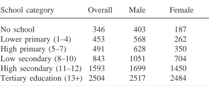
5. Earnings differentials
Table 1 shows average earnings of workers in the HIES sample by levels of education. As expected, aver-age earnings increase as the level of education rises. Males with post-secondary education earn six times more than those with no formal education. The earnings differentials are more pronounced for female employees where those with post-secondary education earn 13 times more than those with no formal education. Compared with earnings differentials reported in 1972 and 1986 (4.5 and 6.1, respectively), these ratios indicate an increase in earnings differentials between those with lower levels of education and those with higher levels of education.5 Females on average earn less than their
male counterparts for all education levels, but the inequality between gender becomes progressively less as education rises. The ratios rise from 0.46 between those with no schooling to 0.98 between those with tertiary education. Gender discrimination, if present, is likely to be at the lower levels of education, especially among those with no schooling and lower primary school level. This might be due to job segregation on a gender basis, especially as there is a stricter division of labour for jobs mainly performed by this category of workers.
Table 2 shows some of the characteristics of workers by type of organisation. The public sector workers are much older, have more years of experience on the job, more years of schooling, and half of them have had some training. Public sector workers also earn more than priv-ate sector employees. The higher average gross earnings of public sector workers could result from the fact that the Government can afford to pay more. The higher aver-age earnings of public sector workers can also be explained by the fact that workers employed in this sec-tor possess more of the human capital stock of schooling,
Table 1
Mean monthly earnings of workers by education levels (Pula): overall and by gendera
School category Overall Male Female
No school 346 403 187
Lower primary (1–4) 453 568 262
High primary (5–7) 491 628 350
Low secondary (8–10) 843 1051 704 High secondary (11–12) 1593 1699 1450 Tertiary education (13+) 2504 2517 2484
a Source: Household Income and Expenditure Survey data,
1993/94.
5 See Kann, Ahmed, Chilisa, Dikole, King, Malikongwa,
Table 2
Characteristics of workers by ownership of organisation/firma
Variable/sector Age Educ. head Experience Hours School Training Gross incomeb
Private sector 31 7.5 8.4 196 7.8 0.33 P736
Public 34 9.4 10.5 169 9.5 0.5 P1115
a Source: Supplementary Survey data.
b Gross earnings is average Pula amount per month from the Supplementary Survey data.
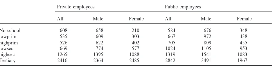
Table 3
Earnings by level of education, by sector and gendera
Private employees Public employees
All Male Female All Male Female
No school 608 658 210 584 676 348
lowprim 535 609 303 667 972 438
highprim 526 622 402 705 809 455
lowsec 669 774 577 1024 1105 953
highsec 1265 1395 1088 1319 1541 1083
Tertiary 2416 2364 2485 2842 3491 1967
a Source: Supplementary Survey data.
experience and training than workers in the private sec-tor. However, it is not certain whether the higher earn-ings in the public sector reflect the higher productivity of workers with more human capital stock, or whether those human capital stocks are being merely used as screens without necessarily making public workers more productive than private sector workers. In other words, screening might be prevalent in Botswana’s public sec-tor.
Table 3 shows average earnings by level of education and by type of employment. Average earnings increase as the level of education increases. Except for those with no schooling, public sector employees on average earn more than private sector employees across all education levels. Earnings ratios between those with no education and those with post secondary education are slightly higher between public employees. Results from Kann et al. (1988) show that for those with no education and those with primary education the average salary was higher in government, whereas for those with secondary and tertiary education levels the private sector paid more. Higher salaries in the public sector for employees with secondary and tertiary education compared with the priv-ate sector reflect two things. First, the ‘decompression’ exercise of 1990 increased government salaries for higher level workers quite significantly. Secondly, due to the relative abundance of graduates from secondary and tertiary levels of education, the private sector no longer needs to pay higher wages than the public sector for recruitment purposes.
6. Exploring earnings variation
In this section we report results of earnings functions in order to explain the differences in earnings in the sam-ple by means of differences in the human capital charac-teristics of individuals. The dependent variable is the natural log of net earnings, where net earnings are defined as gross earnings less tax. Gross earnings are defined as cash earnings plus wages in kind. Earnings are the money plus in-kind payments reported for the month preceding the survey period. The independent variables are schooling, training and experience. For the HIES data, experience is approximated in the usual way as Age-7 for those whose education exceeds 7 years of schooling and Age-14 for those whose education com-prises 7 years or less. Age-14 is a correction aimed at avoiding overestimating potential experience for those with fewer years of education.6The supplementary
sur-vey data include the actual number of years of experi-ence reported by the respondent.
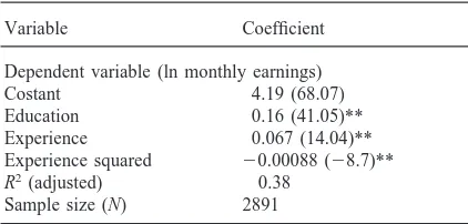
Table 4 summarises the basic earnings function using HIES data. All the coefficients are significant at the 1% level and have the right signs. The model explains 38% of the variations in earnings. The explanatory power of the model is quite robust and is quite comparable, if not slightly better than, some of the results that have used
6 See Dougherty and Jimenez (1991) for further discussion
Table 4
Mincerian earnings function: overall (HIES)a
Variable Coefficient
Dependent variable (ln monthly earnings)
Costant 4.19 (68.07)
Education 0.16 (41.05)**
Experience 0.067 (14.04)**
Experience squared 20.00088 (28.7)**
R2(adjusted) 0.38
Sample size (N) 2891
a Values in parentheses are t-statistics. **, Significant at the
1% level.
this basic earnings function on developing countries (for instance, Kugler & Psacharopoulos, 1989; Psacharo-poulos & Steire, 1988; Al-Qudsi, 1989). The education coefficient, which is also the average rate of return to education is 16%. Experience adds positively to earnings until 38 years on the job, beyond which it contributes negatively to earnings.7
The results presented in Table 4 are, however, poten-tially subject to a type of selection bias. The results are based on an equation estimated from data from only those who were working, resulting in a censored sample of the population. The problem is that the unobserved wage offers of those not working are probably lower than those for persons in the sample. To correct for this we use Heckman’s technique.8This involves a two-step
pro-cess. In the first step the probability that an individual will be gainfully employed and out of school is determ-ined according to a probit regression equation in which a series of personal characteristics serve as regressors. These are age, education and marital status. The probit results are reported in Table A1 in Appendix A. From this probit equation a selection variable, the Inverse Mills Ratio, is created and inserted into the right-hand side of the earnings function. That equation is then re-estimated for those employed to yield estimates free of censoring bias. To correct the estimates for heteroskedasticity we use White (1980, 1993) Heteroskedasticity–Consistent covariance matrix estimation.
The results for the corrected estimates are reported in Table 5. The results of this correction are that the aver-age rate of return to education (which is the expected average rate of return) is lower by 4%. The explanatory power of the model improves significantly. It is also worth noting that the inverse Mill term is significant even at the 0.1% level. The selectivity term is negative,
7 The point where experience stops adding positively to
earnings is defined by∂ln Y/∂T=0, from the earnings function: ln Y=a+bS+cT+dT2. This is equal to c/22d; d,0.
8 See Heckman (1979) for a discussion of this problem.
Table 5
Mincerian earnings function: overall — corrected for censoring bias (HIES)a
Variable Coefficient
Dependent variable (ln monthly earnings)
Constant 5.7 (47.1)
Education 0.12 (26.5)**
Experience 0.009 (1.5)
Experience squared 20.00012 (21.1) Inverse Mills Ratio 21.3 (214.9)**
R2(adjusted) 0.41
Sample size (N) 2891
a Values in parentheses are t-statistics. **, Significant at
1% level.
implying that the observed wage is lower than the wage offers of a randomly selected individual in the popu-lation. The second implication is that those who are in full time employment do not necessarily have a compara-tive advantage.
In Table 6 we fit the Simple Mincerian earnings func-tion with continuous educafunc-tion between male and female workers using HIES data. The results show that the model has a better explanatory power for females with an R2of 51% when fitted on female workers. All
coef-ficients are significant at the 1% level of significance and have the right signs for both sexes. Females have a higher average rate of return of 18% compared with that of males, which is 12%. These paradoxical results are observed in most studies and are attributed to the lower foregone earnings of females compared with their male counterparts (see, for instance, Psacharopoulos & Alam, 1991; Gomez-Castellanos & Psacharopoulos, 1990; Psa-charopoulos, Velez & Patrinos, 1994; Kugler & Psachar-opoulos, 1989). The high private rates of return to females also explain why females have a higher demand for education than males as evident from their higher average years of education. Table 1 also confirms these results, as the average earnings of females are less than those of their male counterparts. The Inverse Mills Ratio is significant at the 0.1% level.
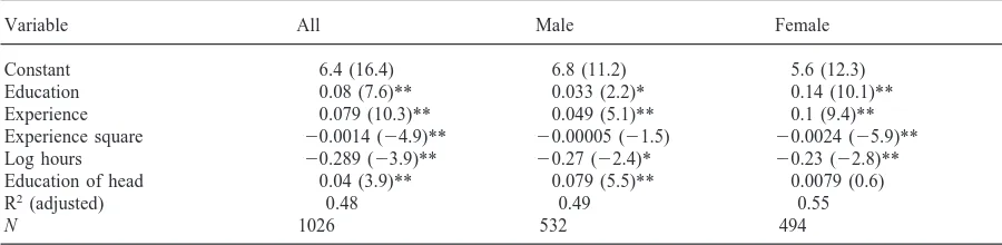
Table 7 explores the effect of adding hours of work and family background variables. Family background is approximated by the education of the head of the house-hold. For all employees, all coefficients are significant at the 1% level of significance and the explanatory power of the model improves slightly by one percentage point. The coefficient of the education of the head of the house-hold is only significant at 1% level of significance for males; it is not significant for females.
Table 6
Mincerian earnings function by gender (HIES)a
Variable Male Female
Dependent variable (ln monthly earnings)
Constant 5.67 (42.1) 4.8 (26.3)
Education 0.12 (22.4)** 0.18 (22.9)**
Experience 0.037 (5.4)** 0.018 (2.08)*
Experience squared 20.0006 (24.8)** 20.0003 (22)*
Inverse Mills Ratio 21.29 (211.3)** 20.98 (29)**
R2(adjusted) 0.47 0.51
Sample size (N) 1587 1304
a Values in parentheses are t-statistics. Asterisks indicate the level of significance: **, 1% level: **, 5% level.
Table 7
Mincerian earnings function with log hours and family background variables (SS data)a
Variable All Male Female
Constant 6.4 (16.4) 6.8 (11.2) 5.6 (12.3)
Education 0.08 (7.6)** 0.033 (2.2)* 0.14 (10.1)**
Experience 0.079 (10.3)** 0.049 (5.1)** 0.1 (9.4)**
Experience square 20.0014 (24.9)** 20.00005 (21.5) 20.0024 (25.9)**
Log hours 20.289 (23.9)** 20.27 (22.4)* 20.23 (22.8)**
Education of head 0.04 (3.9)** 0.079 (5.5)** 0.0079 (0.6)
R2(adjusted) 0.48 0.49 0.55
N 1026 532 494
a Values in parentheses are t-statistics. Asterisks indicate level of significance: **, 1% level; *, 5% level.
environment; (ii) better contacts, leading to good jobs in the labour market. Given that unemployment is quite high, especially for primary and lower secondary edu-cation graduates, it is very likely that family contacts are becoming an important way of learning about and getting a good job. Those with more educated parents are more likely to get better information about employment and therefore obtain better paying jobs.
As shown in Table 7, hours of work have a paradoxi-cal negative coefficient for both male and female work-ers. This seems to suggest that those who supply more hours tend to earn less on average or that low paying jobs are also those that require long hours, e.g. secur-ity guards.
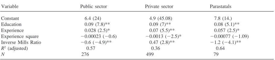
Table 8 presents the results of fitting the Mincerian earnings function to three sectors of Botswana’s econ-omy: the public, private, and parastatal sectors. We cor-rect for choice of employment among the three sectors. The model performs better for the public and parastatal sectors, explaining more than 50% or more of the vari-ation in earnings in those sectors. The explanatory power of the model is, however, relatively weak in the private sector. For the private sector, the model explains about
Table 8
Basic Mincerian earnings function by sector of employment — corrected for choice of employment (SS Data)a
Variable Public sector Private sector Parastatals
Constant 6.4 (24) 4.9 (45.08) 7.8 (14.)
Education 0.09 (7.8)** 0.09 (7)** 0.08 (5.1)**
Experience 0.028 (2.5)* 0.07 (5.5)** 0.057 (2.5)*
Experience square 20.00023 (20.6) 20.0013 (22.5)* 20.00077 (21.09) Inverse Mills Ratio 20.6 (24.9)** 0.47 (2.8)** 21.2 (24.1)**
R2(adjusted) 0.57 0.36 0.64
N 276 499 79
a Values in parentheses are t-statistics. Asterisks indicate level of significance: **, 1% level; *, 5% level.
variable is significant at the 1% level for all three sectors.9
7. Private rates of return to education
Table 9 summarises the results of a Mincerian earn-ings function that has education as a non-continuous variable. We now have 1–0 dummies for the five school-ing cycles.10 All coefficients are significant at the 1%
Table 9
Earnings function with schooling cycles dummies — corrected for censoring bias (HIES)a
Variable All
Constant 5.07 (35.8)
Primary 0.4 (9.7)**
Lower secondary 1.1 (23.3)** High secondary 1.9 (28.8)**
Tertiary 2.1 (21.9)**
Experience 0.057 (7.7)**
Experience square 20.00095 (27.4)** Inverse Mills Ratio 20.78 (26.6)**
R2(adjusted) 0.44
Sample size (N) 2891
a Values in parentheses are t-statistics. **, Significant at
1% level.
9 Refer to Appendix A, Table A2, for probit results for
choice between sectors of employment.
10 Primary education takes 7 years, lower secondary 3 years,
upper secondary 2 years and university 4 years, except for a Degree in Law.
level and have the right signs. Table 10 is a summary of the private rates of return to the different schooling cycles, which are derived from Table 9. The rate of return is highest for upper secondary (185%), then lower secondary (84%) and lowest for primary education (7%).
8. Summary of results and conclusions
The general results from the previous analysis are that the rates of return to education do not decline by level of education. They are highest for upper secondary edu-cation, and lowest for primary education. The general trend, based mainly on Latin American countries and the aggregate ones reported by Psacharopoulos, is for the rates of return to be highest for primary followed by sec-ondary and lowest for tertiary education. Our results also show that the rates of return to the two secondary school education cycles are quite distinct. Higher secondary education has higher private rates of return than lower secondary.
The rates of return to education figures from this study, particularly for primary education, are quite low compared with those estimated by the USAID (1984) study. It is evident therefore that private rates of return to education have been declining, especially for lower secondary and primary education cycles. The falling rates are quite expected given the dramatically changing
Table 10
Annual private rate of return to schooling for each schooling cycle with dummies (%)a
Education Primary Lower Upper Tertiary
level secondary secondary
Rate of 7 83 185 38
return
labour market conditions, particularly on the supply side. There was a significant increase in the supply of gradu-ates (as proxied by total student enrolment) to the labour market, while job opportunities rose less fast. In other words, the rate of employment creation was not adequate to absorb all the graduates entering the labour market. The latest figure on unemployment is estimated at 21% and is highest for those under 25 years of age. It is also highest for those with 1–3 years of secondary education, followed by those with primary education (Republic of Botswana, 1996).
The result of this mismatch between supply and demand for labour was that competition for the few available jobs became intense. The competition created more demand for education at all levels. The labour mar-ket responded to the increases in supply of graduates by escalating minimum job requirements. The result is that school leavers are filtering down occupation hierarchies. For instance, jobs that were previously the preserve of illiterates and primary school graduates are now com-peted for by secondary school graduates.
Although rates of return are generally low, primary education is the most affected. These rates are low because the earnings differentials between workers with primary education and those with no education are very small. Therefore, monetary benefits of going to primary school are very small. This is a result of a phenomenon which has already been discussed: that the primary school graduates were being pushed out of the labour market to very low-paying jobs including informal activities. There are of course some major non-monetary benefits to primary education, which this model does not capture; for instance political awareness, health, etc. Moreover, the benefits for primary education are cap-tured as benefits to other levels of education for those who go beyond primary education.
While lower secondary expanded at a very fast pace, upper secondary education expanded at a relatively lower pace. About 30% or less of the lower secondary completers got places into upper secondary (Republic of Botswana, 1993). It was this group of graduates who were obtaining an increasing share of the mainly skilled, middle level jobs that used to be the preserve of lower secondary school leavers. The additional cost of acquir-ing this privileged access to relatively few good job openings was usually only 2 more years of full time edu-cation. The net income benefits (as shown by the earn-ings differential between this group and the lower sec-ondary school) have been quite high.
Tertiary education has also been highly profitable, as shown in the results from the HIES data. This is mainly due to high earnings compared to earnings of those with upper secondary education level.
Generally rates of return to education increase by level of education. Apart from the changes in the labour mar-ket that have already been discussed, these results may
have other major implications about education. First, that more able people obtain more schooling. The higher rates for higher levels will therefore be a result of higher ability. Second, that quality of education may be improv-ing as one moves up the education ladder. However, this study does not measure changes in school quality and ability differences. Therefore, it is not possible to be pre-cise about the changes in ability and school quality. A more important issue arising from these results is that the British-type of schooling usually contains a strong filtering and screening mechanism through which more able students, or students from households at the higher end of the income distribution, transit up the educational hierarchy. Guisinger, Henderson and Scully (1984) make a similar point about the positive relationship between rates of return and level of education for Pakistan.
Finally, education in Botswana appears to exacerbate income inequalities. The high rate of return for higher levels of education indicate that the distance between the earnings of the highest and lowest worker in the skill hierarchy is large, which may be one reason why Bots-wana has such a high income inequality.11
9. Policy implications
The results from this study have the following policy implications for education and the labour market in Bots-wana.
9.1. Policy implication 1
The rising pattern of private rates of return to edu-cation by level of eduedu-cation suggests that there exists some room for private financing at university level and upper secondary education levels. A shift of part of the cost burden from the state to the individual and his/her family is not likely to create a disincentive of investing in upper secondary and higher education given the high private rates of return to education for these levels of education. The Botswana Government has started to implement a cost recovery programme at tertiary level of education in the form of grant/loan scheme. The results indicate that such a programme could be extended to the upper secondary school level of education. This could reduce expenditure on education quite substantially.
9.2. Policy implication 2
As Botswana’s economy developed and the education system expanded the rates of return to education fell.
11 The 1993/94 Household Income and Expenditure Survey
This was mainly due to a mismatch between demand and supply for labour. If supply continues to outstrip demand we would expect the rates of return to fall further in the future. The high profitability of upper secondary edu-cation might for instance not be sustainable, as tertiary education graduates will be pushing them out to lower paying jobs as the job market tightens up. As educational qualifications continue to be devalued in the labour mar-ket, there is likely to be (as is already evident) increased pressure for more places at the upper secondary and ter-tiary education levels. This means that employment cre-ation has to be pursued very vigorously. It is very costly both economically and politically to have a large number
Table 11
Probit regression of employment status, all and by gender (HIES data)a
Variable All Male Female
Intercept 20.23 20.47 20.49
(23.3) (20.53) (23.9) Age2 (25–34) 0.8 (14.4)** 0.63 (8.4)** 0.92
(12.3)** Age3 (35–44) 1.09 0.84 1.3 (12.7)**
(14.9)** (8.08)**
Age4 (45–54) 1.25 0.89 (6.8)** 1.7 (9.5)** (12.1)**
Age5 (55+) 1.03 (7.3)** 0.67 (3.9)** 1.6 (5.4)** Primary 0.07 (0.9) 0.037 (0.45) 0.13 (1.1) Lower secondary 0.16 (2.1)* 0.15 (1.6) 0.26 (2.1)* High secondary 0.31 (3.3)** 0.29 (2.3)* 0.4 (2.7)** Tertiary 1.4 (4.9)** 1.5 (3.6)** 1.5 (3.5)** Married 0.4 (5.6)** 0.56 (5.5)** 0.3 (2.9)** Log likelihood ratio 646.02 283.02 380.02
Sample size 4056 2144 1912
a Values in parentheses are t ratios. Asterisks give the level
of significance: *, 1% level; **, 5% level.
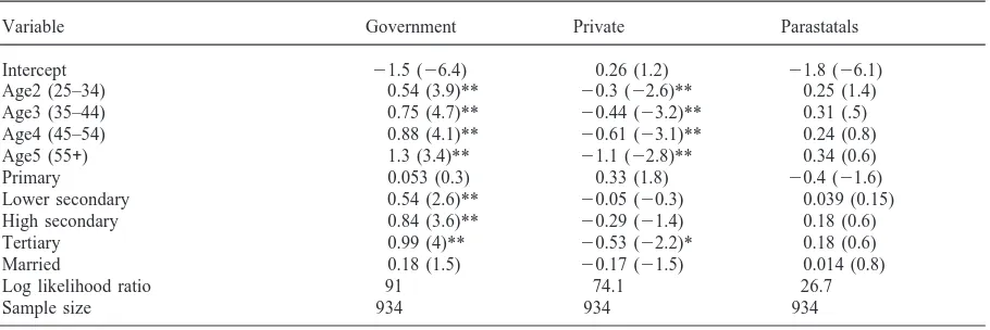
Table 12
Probit regression for choice of employment, government, private and parastatals (SS data)a
Variable Government Private Parastatals
Intercept 21.5 (26.4) 0.26 (1.2) 21.8 (26.1)
Age2 (25–34) 0.54 (3.9)** 20.3 (22.6)** 0.25 (1.4)
Age3 (35–44) 0.75 (4.7)** 20.44 (23.2)** 0.31 (.5)
Age4 (45–54) 0.88 (4.1)** 20.61 (23.1)** 0.24 (0.8)
Age5 (55+) 1.3 (3.4)** 21.1 (22.8)** 0.34 (0.6)
Primary 0.053 (0.3) 0.33 (1.8) 20.4 (21.6)
Lower secondary 0.54 (2.6)** 20.05 (20.3) 0.039 (0.15)
High secondary 0.84 (3.6)** 20.29 (21.4) 0.18 (0.6)
Tertiary 0.99 (4)** 20.53 (22.2)* 0.18 (0.6)
Married 0.18 (1.5) 20.17 (21.5) 0.014 (0.8)
Log likelihood ratio 91 74.1 26.7
Sample size 934 934 934
a Values in parentheses are t ratios. Asterisks give the level of significance: *, 1% level; **, 5% level.
unemployed workers who are highly educated. Given their education, they are more likely to be politically conscious and can cause political upheavals. Moreover, a lot of resources are used to produce these graduates.
9.3. Policy implication 3
The results show that equity is an important issue to consider in implementing cost reduction or cost-sharing schemes in education. Parental background was shown to be an important determinant of schooling and earnings. It is therefore important that a system to identify those from poor backgrounds be put in place. This will enable the Government to identify those eligible for bursaries when school fees are instituted at upper secondary level.
Acknowledgements
This paper draws upon part of my Ph.D. thesis at the University of Manitoba. I wish to thank Professors H. Rempel and W. Simpson for their comments on an earl-ier draft and two anonymous referees for their extensive comments on the paper. I also wish to acknowledge AERC for funding the research and CSO for proving the data. Any errors, of course, are solely my responsibility.
Appendix A
Tables 11 and 12
References
Bennel, P. (1996). Rates of return to education: does the con-ventional pattern prevail in Sub-Saharan Africa? World Development, 24 (1), 183–199.
Colclough, C., & McCarthy, S. (1980). The political economy of Botswana: a study of growth and distribution. (First edition). London: Oxford University Press.
Dougherty, C., & Jimenez, E. (1991). The specification of earn-ings functions: tests and implications. Economics of Edu-cation Review, 10 (2), 85–98.
Gomez-Castellanos, L., & Psacharopoulos, G. (1990). Earnings and education in Ecuador: evidence from the 1989 update. Economics of Education Review, 9 (3), 219–227.
Guisinger, S., Henderson, J., & Scully, G. (1984). Earnings, rates of return and the earnings distribution in Pakistan. Eco-nomics of Education Review, 3 (4), 257–267.
Halvorsen, R., & Palmquist, R. (1980). The interpretation of dummy variables in semilogarithmic equations. American Economic Review, 70, 474–475.
Harvey, C., & Lewis, S. R. Jr. (1990). Policy choice and devel-opment in Botswana. (First edition). London: Macmillan. Heckman, J. (1979). Sample selection bias as a specification
error. Econometrica, 47, 154–161.
Kann, U., Ahmed, G., Chilisa Dikole, R., King, J., Malikongwa, D., Marope, M., & Shastri, G. (1988). Education and employment in Botswana, unpublished research report. Kugler, B., & Psacharopoulos, G. (1989). Earnings and
edu-cation in Argentina: an analysis of the 1985 Buenos Aires Household survey. Economics of Education Review, 8 (4), 353–365.
Mincer, J. (1974). Schooling, experience, and earnings. National Bureau of Economic Research, Columbia Univer-sity Press.
Psacharopoulos, G. (1981). Returns to education: an updated international comparison. Comparative Education, 17 (3), 321–341.
Psacharopoulos, G. (1985). Returns to education: a further inter-national update and implications. Journal of Human Resources, 20, 583–604.
Psacharopoulos, G. (1989). Time trends of the returns to
edu-cation: cross national evidence. Economics of Education Review, 18 (3), 225–231.
Psacharopoulos, G. (1994). Returns to investment in education: a global update. World Development, 22 (9), 1325–1343. Psacharopoulos, G., & Alam, A. (1991). Earnings and education
in Venezuela: an update for the 1987 Household survey. Economics of Education Review, 10 (1), 29–36.
Psacharopoulos, G., & Steire, F. (1988). Education and the labor market in Venezuela, 1975–1984. Economics of Edu-cation Review, 7 (3), 321–332.
Psacharopoulos, G., Velez, E., & Patrinos, H. (1994). Education and earnings in Paraguay. Economics of Education Review, 13 (4), 321–327.
Republic of Botswana (1991). National development Plan 7. Gaborone, Botswana: Government Printer.
Republic of Botswana (1993). Report of the National Com-mission on Education 1993. Gaborone, Botswana: Govern-ment Printer.
Republic of Botswana (1996). Stats brief — unemployment 1991–1994. Botswana Government Printer, Gaborone, Bots-wana.
Republic of Botswana (1999). Budget speech. Gaborone, Bots-wana: Government Printer.
United States Agency for International Development (1984). Botswana: education and human resources sector assess-ment. Mimeo. Washington, DC: USAID.
White, J. (1980). A heteroskedasticity–consistent variance matrix estimator and direct test for heteroskedasticity. Econometrica, 48 (4), 817–838.
White, J. (1993). Shazam user’s reference manual version 7.0. Canada: Ronalds Printing. Second print.
World Development Report 1994: infrastructure for develop-ment. New York: Oxford University Press.
For further reading