www.elsevier.com / locate / econbase
External sector and income inequality in interdependent
economies using a dynamic panel data approach
a b,c ,
*
´
´
Cesar Calderon , Alberto Chong
a
Department of Economics, The University of Rochester, Rochester, NY, USA b
Research Department, Inter-American Development Bank, Stop W-0436, 1300 New York Ave. NW, Washington,
DC20577, USA c
Public Policy Institute, Georgetown University, Georgetown, SC, USA
Received 17 May 2000; accepted 7 November 2000
Abstract
By using a panel of countries for 1960–1995 we show that the intensity of capital controls, the exchange rate, the type of exports, and the volume of trade appear to affect the long run distribution of income. 2001 Elsevier Science B.V. All rights reserved.
Keywords: Income inequality; Globalization; Dynamic panel data
JEL classification: D30; F10
1. Introduction
It has been widely recognized that in recent years the world economies have become more interdependent. Indeed, academics and policymakers broadly agree on the potential gains from trade of this expanded ‘global market’ and on the increased benefits it may bring to the agents. However, it has also become clear that, now more than ever, external conditions in one country may negatively affect other countries’ economies. Awareness of this has been heightened by recent crisis in some parts of the world, particularly in East Asia and Latin America. In this context, one of the greatest concerns of policymakers, especially in middle and low-income countries, is the potential impact of external factors and world trends on the distribution of income. The idea of this note is to empirically address this question trying to assess not only the link itself, but also its extent, by using a wide array of external sector measures. To do this we use an unbalanced panel data set of countries which has
*Corresponding author. Tel.: 11-202-623-1536; fax:11-202-623-2481.
E-mail address: [email protected] (A. Chong).
been organized in 5-year averages for the period 1960–1995 and apply a class of estimators that helps control for country heterogeneity and especially for problems of joint endogeneity of the explanatory variables, a rather common shortcoming in previous empirical work related with several international trade and finance, and development issues.
In the context of the Heckscher–Ohlin model studies that link trade liberalization and wage inequality are not unusual (Cline, 1996). However, here we want to obtain a picture of key external sector measures on household income distribution, not just wage inequality. The connection between skill based wage inequality and income inequality is not necessarily close. Tax issues, number of wage-earners in the household, and additional income sources, are all reasons why this may be true (Wood, 1995, p. 466). This is even more clear in the context of a developing country. Wages are measured based on the formal sector even though the informal sector easily accounts for a third or more of the size of an economy (Loayza, 1996). Given the fact that our aim is to study developed as well as developing countries, and since the external sector is of particular concern on the latter, it only seems sensible to use income distribution measures based on household surveys. This note is organized as follows. The next section describes the data. Section 3 describes our methodology based on Arellano and Bover (1995). Section 4 presents the results. Section 5 concludes.
2. Data
The data is grouped in 5-year averages for the period 1960–1995. To ensure proper applicability of our econometric method we dropped countries with four or less total observations. Our dependent variable, household-based income distribution, is from Deininger and Squire (1997). Our explanatory variables of interest are: (i) terms of trade defined as the log of ratio of exports to import prices; (ii) effective real exchange rate; (ii) Sachs and Warner (1995) external indicator; (iii) volume of trade, defined as the sum of exports plus imports of goods and services, as a ratio of GDP; (iv) ratios of exports of non-fuel primary commodities and manufacturing goods as a percentage of total exports; (v) balance of payments restrictions from Grilli and Milesi-Ferreti (1995), and (vi) black market
1
premium on foreign exchange . Following previous literature, additional controls are liquid liabilities, schooling, and initial GDP per capita in each 5-year period considered (Li et al., 1998; Chong, 2000).
3. Econometric approach
Our econometric model is dynamic (in the sense that the explanatory variable set includes a lag of the dependent variable) and includes some explanatory variables that are potentially jointly endogenous (in the sense of being correlated with the error term). In addition, the model presents an unobserved country-specific factor that is correlated with the explanatory variables. In order to estimate our model consistently and efficiently, we use a GMM estimation for dynamic panel data models (Arellano and Bover, 1995) that encompasses a regression equation in both differences and
1
levels, each one with its specific set of instrumental variables. The general regression model for income inequality follows:
yi,t5b1 yi,t211b2Xi,t1hi1´i,t (1)
We eliminate country-effects (hi) by expressing (1) in first-differences:
yi,t2yi,t215b1
s
yi,t212yi,t22d
1b2s
Xi,t2Xi,t21d
1s
´i,t2´i,t21d
(2)We use instruments to control for likely endogeneity of the explanatory variables, X, reflected in the correlation between these variables and the error term. We allow for the possibility of simultaneity and reverse causation by assuming weak exogeneity of the explanatory variables (no correlation with future realization of error term). Additionally, we assume that the error term, ´, is not serially correlated and apply:
E y
f
i,t2s?s
´i,t2´i,t21dg
50 for s$2; t53, . . . ,T (3)E X
f
i,t2s?s
´i,t2´i,t21d
g
50 for s$2; t53, . . . ,T (4)The resulting GMM estimator is known as the difference estimator. Although asymptotically consistent, it has low asymptotic precision and large biases in small samples, which leads to the need of complementing it with a regression equation in levels. Applying this does not eliminate directly the country-specific effect but controls it when using instruments. The appropriate instruments are the lagged differences of the corresponding variables, under the assumption that, although there may be correlation between levels of the right-hand side variables and the country-specific effect, none exists between the differences of these variables and the country-specific effect. This results from the following stationarity property:
E y
f
i,t1p?hig
5E yf
i,t1q?hig
andf
Xi,t1p?hig
5E Xf
i,t1q?hig
for all p and q (5)The additional moment conditions are:
E y
fs
i,t2s2yi,t2s21d s
?hi1´i,tdg
50 for s51 (6)E X
fs
i,t2s2Xi,t2s21d
?s
hi1´i,td
g
50 for s51 (7)We use the above equations and a GMM procedure to generate consistent estimates of the parameters of interest. We use a Sargan test of over-identifying restrictions to test the overall validity of the instruments. Additionally, a second test examines whether the differenced error term is serially correlated.
4. Results
Our basic reduced form follows:
GIN 5a1bGIN 1fGDP 1dEDU 1hLLQ 1nEXT 1´ (8)
Where GIN is the Gini coefficient in period t for country i, GINit it21 is the lagged Gini coefficient,
GDP is the (log of) real GDP per capita, EDU is the fraction of the population with completeit it
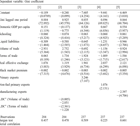
primary education, LLQit are liquid liabilities as a percentage of GDP, and EXTit is a vector that contains indicators related with the external sector (volume and terms of trade, real exchange rate, black market premium, and capital controls). The explanatory variables are allowed to be jointly weakly endogenous. Table 1 reports our main results. The Sargan test of overidentifying restrictions does not reject the null hypothesis that the instruments are not correlated with the error process. Also, tests of serial correlation fail to reject the null that the error term, expressed in first differences, is not second- or third-order serially correlated while, by construction, accepts the null that this process
Table 1
Dependent variable: Gini coefficient
[1] [2] [3] [4] [5]
Constant 20.189 20.248 27.605 29.441 26.469
2(0.0789) 2(0.099) 2(4.254) 2(4.163) 2(3.010)
Gini lagged one period 0.884 0.925 0.855 0.896 0.864
(72.892) (45.570) (64.126) (69.825) (68.704) Domestic GDP per capita 0.151 2(0.137) 0.520 0.667 0.554
(1.119) 20.775 (6.344) (6.856) (5.957)
Schooling 20.060 20.074 20.063 20.060 20.061
2(8.324) 2(8.416) 2(5.217) 2(4.925) 2(5.289) Liquid liabilities 20.309 20.588 20.645 21.231 20.946
2(1.464) 2(2.585) 2(1.873) 2(4.657) 2(2.708)
Volume of trade 22.931 2.752 20.692 21.156 20.924
2(5.364) (1.543) 2(2.115) 2(3.347) 2(2.994)
Terms of trade 0.063 1.734 21.924 21.089 21.586
(0.189) (1.246) 2(3.121) 2(1.715) 2(2.617)
Real effective exchange 1.076 1.319 1.941 2.037 2.121
(3.883) (3.929) (6.734) (6.299) (6.898) Black market premium 20.002 20.002 20.003 20.002 20.005
2(7.315) 2(4.676) 2(8.516) 2(3.682) 2(5.354)
LDC (Volume of trade) 2(8.005) 22.851 a
LDC (Terms of trade) 2(2.361) 21.220
Observations 284 284 237 237 237
Sargan test 0.437 0.470 0.589 0.225 0.601
Serial correlation
First-order 0.019 0.027 0.040 0.024 0.035
Second-order 0.419 0.499 0.979 0.705 0.882
Third-order 0.979 0.923 0.733 0.874 0.828
a
exhibits first-order serial correlation. This gives support to using lags of the explanatory variables as instruments.
Bearing in mind that a positive sign in the corresponding coefficient indicates a worsening in the distribution of income we find that, with respect to typical core controls, our results yield similar results to previous studies. In fact, increased financial deepening, as proxied by liquid liabilities, reduces inequality (Li et al., 1998); also, past inequality appears to be an important predictor of current inequality (Chong, 2000). Our results confirm that schooling appears to reduce income
´
inequality (Chong and Calderon, 2000; Squire, 1998). On the other hand, with respect to our variables of interest, we find that: (i) a 5% increase in the volume of trade leads to a long-run decline of 1.26 points in income inequality, as reflected by a decrease in the Gini index (column 1). Also, when controlling for the size of primary or manufacturing exports, the coefficient becomes smaller but keeps high significance. We find that export orientation towards primary activities may be associated to higher income inequality while export orientation towards manufacturing goods may be linked with lower inequality. This appears to be somewhat consistent with the hypothesis of enclaves, by which primary activities do not produce extensive linkages to the local economy so that that inequality between the elite and the rest of the society may increase; (ii) the impact of the terms of trade is statistically insignificant in our core regression (column 1). However, the relationship becomes significant when controlling for type of exports (columns 3–5); (iii) a real depreciation of the local currency reduces the Gini coefficient, possibly as a result of gains in competitiveness. A 10% real depreciation of the local currency helps decrease income inequality by 0.9 points (column 1). This increases to 1.3–2.0 points if we control for the orientation of exports; (iv) we find a negative and significant relationship between intensity of balance of payments controls, as expressed by distortions in the foreign exchange market (black market premium) and income inequality. The impact is very small, though. Similarly, even though, as mentioned above, we do not necessarily expect to find results consistent with the Heckscher–Ohlin prediction we, however, use interactive dummies in order to test whether variables such as the volume of trade and the terms of trade have opposing effects with respect to income inequality depending upon whether the country is developed or underdeveloped (column 2). We find that while the impact of volume of trade (‘openness’) is positive and barely statistically significant for industrial countries, it is negative and statistically significant for developing countries (column 2). This is somewhat consistent with the Heckscher–Ohlin theorem. An increase of 5% in the volume of trade is linked with a long-run decline of 3.5 points in income inequality, while such a decline was only 1.3 points in the core regression (column 1). Finally, with respect to terms of trade we find that the link is not significant when we separate the effects even though the sign of the
2
coefficient of the interactive term differs, as expected .
5. Conclusions
It appears that the volume — but not the terms — of trade, the real exchange rate, and the intensity — and not just the presence — of capital controls are associated with changes in income distribution.
2
The type of exports appears to matter as primary export countries, of which most are developing ones, are associated with an increase in inequality, while manufacturing export ones, of which most are developed, are linked with decreasing inequality. Finally, with respect to volume of trade, our findings are somewhat consistent with the Heckscher–Ohlin hypothesis.
Acknowledgements
The opinions are the authors’ and should not be attributed to the Inter-American Development Bank.
Appendix. Countries in sample
Africa 36. Canada 71. Malaysia
01. Algeria 37. Costa Rica 72. Nepal
02. Botswana 38. El Salvador 73. Pakistan
03. Cameroon 39. Dominican R. 74. Philippines 04. C. African R. 40. Guatemala 75. Singapore
05. Congo 41. Honduras 76. Sri Lanka
06. Egypt 42. Jamaica 77. Taiwan
07. Ethiopia 43. Mexico 78. Thailand
08. Gambia 44. Nicaragua
09. Gabon 45. Trinidad and Tobago Europe
10. Ghana 46. United States 79. Austria
11. Guinea 47. Argentina 80. Belgium
12. Guinea-Bissau 48. Bolivia 81. Bulgaria
13. Cote d’Ivoire 49. Brazil 82. Czech Republic
14. Kenya 50. Chile 83. Denmark
15. Lesotho 51. Colombia 84. Finland
16. Madagascar 52. Ecuador 85. France
17. Malawi 53. Guyana 86. Germany
18. Mauritania 54. Panama 87. Greece
19. Mauritius 55. Paraguay 88. Hungary
20. Morocco 56. Peru 89. Ireland
21. Niger 57. Puerto Rico 90. Italy
22. Nigeria 58. Uruguay 91. Netherlands
23. Rwanda 59. Venezuela 92. Norway
24. Senegal 93. Poland
25. Seychelles Asia 94. Soviet Union
26. Sierra Leone 60. Bangladesh 95. Spain
27. South Africa 61. China 96. Sweden
29. Tunisia 63. India 98. Turkey
30. Uganda 64. Indonesia 99. United Kingdom
31. Zambia 65. Iran
32. Zimbabwe 66. Iraq Oceania
33. Tanzania 67. Israel 100. Australia
68. Japan 101. Fiji
Americas 69. Jordan 102. New Zealand
34. Bahamas 70. South Korea 35. Barbados
References
Arellano, M., Bover, O., 1995. Another look at the instrumental variable estimation of error-component models. Journal of Econometrics 68, 29–51.
Cline, W., 1996. Trade and Income Distribution. IIE, Washington, DC.
Chong, A., 2000. Democracy, Inequality, and Persistence: Is There a Political Kuznets Curve. Development Research Group, The World Bank, Washington, DC, Manuscript.
´
Chong, A., Calderon, C., 2000. Institutional Quality and Distribution of Income, Economic Development and Cultural Change, July
Deininger, K., Squire, L., 1997. A new data set measuring income inequality. World Bank Economic Review 10, 565–591. Grilli, V., Milesi-Ferreti, G.M., 1995. Economic effects and structural determinants of capital controls. IMF Staff Papers 42,
517–551.
Li, H., Squire, L., Zou, H.-F., 1998. Explaining international and intertemporal variations in income inequality. Economic Journal 108, 26–43.
Loayza, N., 1996. The economics of the informal sector: a simple model and some empirical evidence from Latin America. Carnegie–Rochester Conference on Public Policy 45, 129–162.
Sachs, J., Warner, A., 1995. Economic reform and the process of global integration. Brookings Papers on Economic Activity 1, 1–95.