VOXEL- AND GRAPH-BASED POINT CLOUD SEGMENTATION OF 3D SCENES USING
PERCEPTUAL GROUPING LAWS
Y. Xu∗, L. Hoegner, S. Tuttas, U. Stilla
Photogrammetry and Remote Sensing, Technische Universit¨at M¨unchen, 80333 Munich, Germany -(yusheng.xu, ludwig.hoegner, sebastian.tuttas, stilla)@tum.de
Commission II, WG II/4
KEY WORDS:Point cloud, Segmentation, Voxel structrue, Graph-based clustering, Perceptual grouping laws
ABSTRACT:
Segmentation is the fundamental step for recognizing and extracting objects from point clouds of 3D scene. In this paper, we present a strategy for point cloud segmentation using voxel structure and graph-based clustering with perceptual grouping laws, which allows a learning-free and completely automatic but parametric solution for segmenting 3D point cloud. To speak precisely, two segmentation methods utilizing voxel and supervoxel structures are reported and tested. The voxel-based data structure can increase efficiency and robustness of the segmentation process, suppressing the negative effect of noise, outliers, and uneven points densities. The clustering of voxels and supervoxel is carried out using graph theory on the basis of the local contextual information, which commonly conducted utilizing merely pairwise information in conventional clustering algorithms. By the use of perceptual laws, our method conducts the segmentation in a pure geometric way avoiding the use of RGB color and intensity information, so that it can be applied to more general applications. Experiments using different datasets have demonstrated that our proposed methods can achieve good results, especially for complex scenes and nonplanar surfaces of objects. Quantitative comparisons between our methods and other representative segmentation methods also confirms the effectiveness and efficiency of our proposals.
1. INTRODUCTION
Point clouds obtained via laser scanner, photogrammetry, and range imaging cameras are widely used to represent 3D spatiality information of scenes, and applied in a wide variety of fields, including geodesy, geomatics, geology, forestry, and archeology. For all the mentioned applications, the 3D scene reconstruction is drawn increasing attention for many related tasks such as constructing virtual reality, creating digital surface models, or monitoring construction projects. In particular, point clouds have been proved to be a suitable data source for the task of recognizing and reconstructing geometric objects from 3D scenes, as 3D points measured can provide 3D coordinates of objects directly. However, for most of the indoor and outdoor scenes, they normally consist of different objects, combinations of complex structures, surfaces, and sections. Thus, in practical, individual objects are commonly identified from the scene prior to the recognition procedure.
To this end, for unstructured raw point clouds, segmentation are normally adopted to partition the 3D scene into meaningful seg-ments (e.g., the group of points having geometric consistency). An effective segmentation algorithm can facilitate the removal of disturbances and largely release the burden of work, but the performance of conventional algorithms is always restrained by the complex environment of real outdoor scenes. The occlu-sion frequently occurring in the dataset of outdoor scene also limit the performance of commonly used methods, as most of the segmentation criteria use merely the pairwise information between elements (e.g., normals of points), which is sensitive to missing points and incomplete structures caused by occlusions. Moreover, the data quality is also a leading cause of inferior
∗Corresponding author
segmentations. For instance, outliers and uneven points den-sity can significantly affect the results resorting to point-based geometric features (e.g., normal vector). Hence, apart from the effectiveness, the reliability plays a vital role in the development of segmentation algorithms as well. On the other hand, as the point cloud segmentation is computationally intensive, efficiency is also crucial to the point cloud processing and should be con-sidered when coping with large-scale datasets.
1.1 Related work
The point cloud segmentation has been studied and explored for decades, with methods and algorithms in different disciplines including computer vision, computational geometry, robotics, photogrammetry, remote sensing, machine learning and statistics exploited (Vosselman and Maas, 2010). Summarily, the relevant point cloud segmentation approaches can be grouped into three major categories: the model-based methods, the region growing-based methods, and the clustering-growing-based methods (Vo et al., 2015).
The model-based methods evaluate the points in terms of their geometric features (e.g., spatial position and normal vector) in a local or global scale using parametric models. The points meeting the criteria of fitting parametric models (either in spatial or parametric domain) are segmented from the point cloud as one individual object. The 3D Hough Transform (HT) (Ballard, 1981) and the RANSAC (Schnabel et al., 2007) are two kinds of widely used algorithms (Vosselman, 2013). The HT and it variations utilize a voting strategy for extracting planes (Vosselman et al., 2004), cylinders and spheres (Rabbani et al., 2006) from the point cloud in the parameter domain. Whereas RANSAC and its extensions directly estimate optimal parameters of the geometric models in spatial domain (Schnabel et al., 2007). The model-based methods commonly deem robust to noise and outliers and provide optimized parameters for modeling simultaneously. Nevertheless, when dealing with large-scale datasets, they nor-mally require nornor-mally a large computational cost caused by the iteration process of robust estimator or the voting procedure, leading to high memory consumptions (Vo et al., 2015). Besides, challenges arise they are used to segment objects having no ex-plicit mathematical expressions like irregular curvature surfaces.
The region growing-based ones iteratively examine points in regions of initial seeds and checks whether they belong to the group of the seed or not via a given criteria. The growing criteria and the selection of seeds are two influential factors for this kind of methods. The normal vectors consistency (T´ov´ari and Pfeifer, 2005), the smoothness of surface (Rabbani et al., 2006), and the curvatures (Besl and Jain, 1988) of the points are commonly used growing criteria. Recently, in Nurunnabi et al., (2012), the Principal component analysis (PCA) based local features are also used as growing criteria for their saliency and distinctiveness. For the selection of seeds, the density of seeds determines the size of segments while the location of seeds significantly affect the quality of segments. The region with the smallest curvature (Nurunnabi et al., 2012) or the surface with minimal residual of a plane fitting (Rabbani et al., 2006) are frequently identified as seeds, in order to avoid the boundaries and edges. Theoreti-cally, region growing-based methods can keep the boundaries of surfaces well, but they are sensitive to noise and outliers. For example, over-segmentation can easily occur for large curvature objects (e.g., pipes with a long radius elbow joint) although the surfaces of which are smoothly connected (Su et al., 2016). On the other hand, their performances largely resort to the selection of seeds (e.g., the location and distribution of seeds).
The last major kinds are the clustering-based ones. This kind of methods examine the neighboring points in a defined neigh-borhood by their proximity or similarities in the attribute or spatial spaces on the basis of the geometric characteristics and spatial coordinates. Points having a proximity or similarity lower meeting the acceptable threshold are assessed as connected ones, which will be aggregated into one cluster. Euclidean distance
(Aldoma et al., 2012) and normal vector (Vo et al., 2015) are representative instances used as criteria for clustering. For the clustering algorithms, the k-means (Morsdorf et al., 2003), mean-shift (Comaniciu and Meer, 2002), and connected relations (Stein et al., 2014) are mostly adopted ones. Unlike region growing-based methods, the clustering-growing-based ones require no seeds. Note that the computational cost of clustering-based methods lies on the complexity of calculating the similarities or proximity of points. Complex clustering criterion will greatly increase the computational burden. Besides, the setting of clustering thresh-olds is also influential to the granularity of clusters segmented.
Recently, there is a tendency that the clustering of points is also formulated as graph construction and partitioning problems. The graph model can explicitly organize the elements (e.g., pixels or points) with a mathematical sound structure (Peng et al., 2013), encapsulating the contextual information for deducing hidden information from the given observations. Representative examples include the graph-based approaches such as Min Cuts (Golovinskiy and Funkhouser, 2009), and Graph segmentation (Green and Grobler, 2015) and the Markov-based approaches like the Markov Random Field (MRF) (Hackel et al., 2016a) or Conditional Random Field (CRF) (Rusu et al., 2009). For graph-based methods, a large topology radius of constructed graphs can provide better results in segmentation, but a dense and large graph yields a heavier computational cost (Cour et al., 2005).
In addition, the voxel-based segmentation methods draw in-creasingly attention recently. Instead of using points as basic units, 3D regular cubes occupied by points are used as basic segmentation elements (Wang and Tseng, 2011). The octree-structured voxelization is the most commonly used approach. In Vo et al., (2015), the octree structure and the region growing process are combined for the fast surface patch segmentation. Whereas, the octree-based voxel structure combined with graph-based sub -splitting is applied to segment cylindrical objects in industrial scenes (Su et al., 2016). Using voxel structure apparently reduces the computation cost and suppress negative effects of outliers and varying point densities. Even so, selecting an appropriate resolution of voxel is crucial to the accuracy of segments and preservation of details. Lately, the supervoxel strategy is introduced and applied to the basic voxel structures, better preserving the boundary features of segments and further improving the computation efficiency (Stein et al., 2014, Pham et al., 2016, Ramiya et al., 2016). However, the supervoxel method is merely an over-segmentation of data, how to cluster over-segmented patches into segments is still a challenging task.
1.2 Our contributions
The following are the contributions that are specific to this work: 1) A bottom-up point cloud segmentation strategy, combing the voxel structure and graph-based clustering encoding the local contextual information, is proposed. Two novel segmentation methods (i.e., VGS and SVGS) are reported, and they are proved to be effective and efficient for 3D scene segmentation. 2) Instead of using conventional criteria, the perceptual grouping laws are adopted to assess geometric cues used in our methods, providing a purely geometric and unsupervised solution for segmentation. 3) Experiments using both laser scanned and photogrammetric point clouds of the same scene are conducted. The performance of proposed methods coping with datasets from different sources is analyzed.
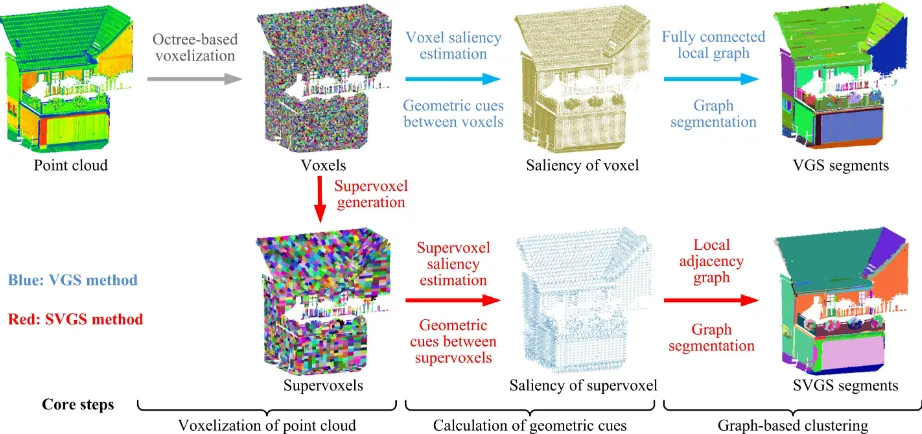
Figure 1. Workflow of voxel- and graph-based segmentation strategy
2. OVERVIEW OF METHODOLOGY
Conceptually, the implementation of our proposed segmentation strategy concerns three core steps: the voxelization of point cloud, the calculation of geometric cues, and the graph-based clustering. In the first step, the entire point cloud is voxelized into the 3D grid structure. For the VGS method, the voxel is the basic unit for segmentation, while for the SVGS method, voxels will be further clustered into supervoxels as basic units, having geometric consistency and spatial dependency. In the subsequent step, in order to estimate the geometric cues between basic units (i.e., voxels or supervoxels), the saliency of each basic unit is calculated by the use of points set within it. Depending on these saliencies, geometric cues between basic units are estimated ac-cording to perceptual grouping laws, so that the affinity between voxels or supervoxels can be assessed by the homogeneities of geometric cues, which will be further used for weighting edges in the graph model. In the last step, the graph-based clustering is conducted to merge voxels or supervoxels in terms of their affinity under a greedy frame, in order to generate complete segments. The graph model is constructed for each basic unit in its vicinity, encoding the local contextual information in the form of adjacency graph. By applying the graph segmentation algorithm, the connectivity of each unit can be estimated, so that all the connected units can be aggregated into complete segments by a simple clustering. The processing workflow is sketched in Fig. 1, with the key steps of involved two methods and sample results illustrated. The detailed explanation of VGS and SVGS methods will be introduced in the following sections.
3. VOXEL- AND GRAPH-BASED SEGMENTATION
The VGS method is the basic solution implemented via our strategy, utilizing the voxel structure and the fully connected local graph, reported in our recent work (Xu et al., 2017).
3.1 Voxelization of point cloud
In this work, we adopt the octree-based voxelization to rasterize the entire point cloud with 3D cubic grids. Under the octree
structure, the nodes have explicit linking relations, which facil-itates the traversal for searching the adjacent ones (Vo et al., 2015). It is noteworthy that selecting the size of voxels is a trade-off between the efficiency of processing and the preservation of details. Generally speaking, the smaller the voxel, more details will be kept. In our work, the size of voxel is determined according to the demands of application empirically.
3.2 Calculation of geometric cues
Geometric cues stand for the geometric relations between two voxels, including two steps: voxel saliency estimation and geo-metric cues using perceptual laws.
3.2.1 Voxel saliency estimation The saliency of each voxel can be regarded as the unary feature of each voxel delineating the points within it, including three factors: the spatial location, the geometric features, and the normal vector of the points.
The spatial position refers to the spatial coordinates of the cen-troidsX~ of points within a voxelV. For geometric features, the eigenvalue based geometric features (Weinmann et al., 2015) are used, delineating the 3D properties of points inside a voxel, re-lated to the local shape features encapsulating the linearityLe, the
planarityPe, the scatteringSe, and the change of curvatureCe
(Weinmann et al., 2015). These four feature sets are calculated via eigenvaluese1 ≥e2 ≥e3 ≥0from eigenvalue decomposi-tion (EVD) of the 3D structure tensor (i.e., covariance matrix) of points coordinates. As stated in Weinmann et al. (2015),
Le, Pe, and Se represent 1D, 2D, and 3D features of points,
respectively, whereas Ce reflects the curvature of the surface.
For the normal vectorN~ of points withinV, it is obtained from the eigen vectors of the points. Considering noise and outliers always existing in point clouds, the estimation of eigenvalues and eigenvectors will be susceptible to such disturbances. We adopt the weighted covariance matrix proposed in (Salti et al., 2014), assigning smaller weights to distant points in the covariance matrix of coordinates.
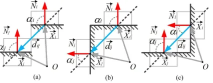
Figure 2. Connection types. (a)“stair-like”, (b) convex, and (c) concave connections.
vision for recognizing objects from the scene, refering to determi-nation of regions of the visual scene belonging to the same part of higher level perceptual units (Richtsfeld et al., 2014). Three representative principles of the grouping laws are selected as our clustering criterion: proximity, similarity, and continuity.
The proximity principle states that elements are likely to be categorized into a same group if they are close to each other. Whereas the similarity principle claims that elements tend to be summed into a group when they resemble each other. For the continuity principle, it indicates that the oriented elements are considered to be integrated into one part in case that they can be aligned with each other.
To measure the proximity ofViandVj, we utilize the Euclidean
distanceDs
ij = ||X~i−X~j||between the centroidsX~iandX~j
ofViandVj. Since the shape similarity denotes the conformity
between the shapes of points within voxels, the stronger the similarity between the geometric features of voxels, the more similar the points within the voxels are. For theDs
ij between
ViandVjin this 4 dimensional feature space is calculated using
the histogram intersection kernel (Papon et al., 2013). For the connectivity, it corresponds to the smoothness (Awrangjeb and Fraser, 2014) and convexity criterion (Stein et al., 2014) formed by the points surfaces of adjacent voxels. In Fig. 2, we illustrate three typical connections between voxels. The smoothness is defined by the angle difference of normal vectors N~i andN~j.
The convexity criterion stands for the 3D concave or convex relationship connecting surfaces formed by the points of two adjacent voxels, inferred from the relation ofN~i and N~j and
the vector d~ij joining their centroids X~i and X~j. As shown
in Figs. 2, the anglesαi andαj are calculated, whered~ij =
(X~i−X~j)/||X~i−X~j||. Ifαi−αj> θ, the surface connectivity
is defined as a convex connection, whereθ is the threshold for convexity judgement. Otherwise, it is a concave connection. Similar to work reported in (Stein et al., 2014), we also assume that for one object the convex connection should be preserved while the concave connection should be disconnected on the basis of the degree of the convexity criterion. The“stair-like”
surfaces (see Fig. 2a) are highly likely to be parts of different objects and should be disconnected. Considering these three situations, the surface connectivityDc
ijis calculated according
to Eq. 1, giving the blunt convex or smooth connected surfaces a higher proximity value, while for the concave connected surfaces a constant penalty so that they are likely to be determined as disconnected. θ is calculated by a sigmoid function determined by the difference ofαiandαj, following the description in (Stein
et al., 2014).
Figure 3. (a) Adjacent voxels in a neighborhood. (b) Fully connected local graph.
3.3 Graph-based clustering
In many former work, the connection of voxels are merely iden-tified by the relation between two adjacent voxels, with their similarity or normal vector used (Wang and Tseng, 2011), (Papon et al., 2013). However, due to the complex environment of the 3D scene, the assessment of connections considering only information a voxel pair seems unreliable. To that end, we introduce the graph theory to assess the connections of a center voxel considering all the neighboring voxels in a neighborhood of the center voxel simultaneously. Thus, a fully connected local graphG= (V, E)is constructed as shown in Fig. 3.
3.3.1 Fully connected local graph For the fully connected local graph, voxels are set as vertices V while the edges E
are linked between all the vertex pairs. For the central voxel, its adjacent voxels belonging to the same group after the graph segmentation are regarded as the connected ones. The weight
wij∈[0,1]betweenViandVjis defined by integrating affinities
Dijbetween voxels calculated via a multiplicative form as they
are independent:
kernel, controlling the importance of the spatial distance, the geometric similarity, and the surface connectivity, respectively. In our cases, all of them are set to 0.1 equally.
3.3.2 Graph-based segmentation Once the graph is con-structed, we can achieve the connection of voxels by optimization method, namely the partition of the graph. For this purpose, the graph-based segmentation method is introduced by adapting the algorithm proposed in (Felzenszwalb and Huttenlocher, 2004). Here, the segmentation C is to partition voxels V (i.e., the vertices in the graph) into segmentsS ∈ Cequating with the connected components in the graph. As the initial step, every vertexViis regarded as one segmentSi. The edges are sorted
in ascending order according to their weights. Then, the graph is partitioned via a recurrently process by comparing the weightw
of an edge with the maximum internal differenceIiof a segment
Si. For verticesVi ∈ SmandVj ∈ Snof an edgeEij, if the
weightwij is larger than the thresholdτmn, then theSmand
Snwill be merged as one segment. Here, the thresholdτmnis
estimated as follows: parameter setting the initial threshold value. In the extreme case, if|Sm|= 1and|Sn|= 1, thenτmn=δ. This merging process
is performed repeatedly by traversing all the edges. In Algorithm. ISPRS Annals of the Photogrammetry, Remote Sensing and Spatial Information Sciences, Volume IV-1/W1, 2017
1, we provide a detailed description. According to the output
Algorithm 1Graph-based segmentation
Input: G= (V, E), Graph with verticesV and edgeE
Output: C= [S1, S2, ..., Sn]: Segments of vertices
0: SortEin ascending order by its weightw
1: Initial segmentationC0= [S
1, S2, ..., Sm],Si= [Vi]
2: Initial thresholdτij=δ,Ii= 0
3: for∀Eij∈Edo
4: Ifwij > τij=max(Ii+|Sδ
i| +
δ
|Sj|)
5: Sk⇐Si∪Sj
6: Ik=wij+|Sδ
k|
7: C⇐ {C\{Si∪Sj}} ∪Sk
of the graph partition, in the neighborhood of a center voxel, its connections can be identified by the group of nodes in the graph.
3.3.3 Clustering of connected voxels Once the connections of all the voxels are identified, the connected voxels are merged into one segment. This merging process is performed repeatedly by traversing all the voxels, with a depth-first strategy. In the neighborhood of a center voxel, its connections can be identified by the group of nodes in the graph, then all the connected voxels are aggregated into one segment. In addition, a cross validation process is carried out to ensure the correctness of connections. For adjacentViandVj, after segmenting the graph ofVi, ifViis
identified as connected toVj, then in the segmentation of graph
ofVj,Vjshould be connected toViin turn. Otherwise, they are
disconnected.
4. SUPERVOXEL- AND GRAPH-BASED SEGMENTATION
The SVGS method is an improved solution utilizing the super-voxel structure and the local affinity graph, improved from our former work (Xu et al., 2016). It has three significant differences compared with the VGS method. Firstly, the supervoxels are used as basic units for clustering into segments, instead of directly using voxels. Secondly, the definition of graph is different. We define a local adjacency graph rather than the fully connected graph used in VGS. At last, the clustering of connected basic units, here, the aggregation of supervoxels is conducted resorting to the merging of adjacency graphs.
4.1 Supervoxel generation
The generation of supervoxels is carried out by the Voxel Cloud Connectivity Segmentation method (VCCS) (Papon et al., 2013), clustering the voxels of points in terms of the distance between the seed and candidate voxels in a feature space, involving geo-metrical features, and RGB colors (Papon et al., 2013). Slightly different from the way described in (Papon et al., 2013), we merely use normal vectors and spatial coordinates of voxels to define the distance, which is related to the proximity and conti-nuity principles. The VCCS we used is implemented and tailored from the Point Cloud Library (PCL) (Rusu and Cousins, 2011). One of the most significant advantage of VCCS is the boundary preservation performance (Papon et al., 2013), so that we can obtain the supervoxels sharing same boundaries with the major structures of objects in the scene. Note that, the size of the voxel and the resolution of seeds can greatly affect the performance of VCCS. The former one determines the details preserved in the scene, while the later influences the effectiveness of keeping boundaries. Empirically, we set these factors according to the densities and the varying range from the sensor to the objects.
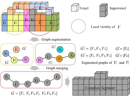
Figure 4. Aggregation of supervoxels.
4.2 Local adjacency graph
To apply the graph model to the supervoxel structure, we define a local adjacency graph for each supervoxel encoding all the neighboring supervoxel in a local vicinity, so that the connectivity of two adjacent supervoxels can be assessed in a context-aware way. In detail, for each supervoxelVi, all itsnneighbors with
a spatial distance between centroids smaller than a given radius
Rcare counted as the candidate ones for building the contextual
graphGi={V, E}, which is represented in the form of nodes.
The spherical space defined byRcis termed as the local context
of each supervoxel. For each node, only these edges connecting its adjacent ones will be considered. The weights of edges
E are estimated by the use of aforementioned geometric cues in a same way like VGS. The partition of the local adjacency graphG is the same like that of VGS, using the graph-based segmentation (Felzenszwalb and Huttenlocher, 2004), by which the segmented graphG+can be obtained. InG+, the connected nodes representing the connectivity of supervoxels.
4.3 Aggregation of supervoxels
To aggregate the supervoxels, all the segmented local adjacency graphs are traversed and checked. For these segmented graphs having common nodes (see Fig. 4, the nodeVk shared by the
graphsG+i andG
+
j), they will be merged into one large graphG,
encoding the connection information of nodes within it. At last, for each merged graphG, all the supervoxels represented by the connected nodes will be aggregated into a complete segment as shown in Fig. 4.
5. RESULTS AND DISCUSSION 5.1 Experimental datasets
HDS 7000, while the photogrammetric point cloud is generated from a structure from motion (SfM) system and multi-view stereo matching method (Tuttas et al., 2014), using a Nikon D3 DLSR camera with 105 images. The statistical outlier removal filtering (Rusu and Cousins, 2011) is applied to the point clouds prior to the main processing. The sizes of LiDAR and photogrammetric point clouds are both around nine million points. To evaluate the performance of our method, four representative segmenta-tion algorithms, including the Euclidean distance and difference of normal (DON) based clustering(Ioannou et al., 2012), the smoothness based region growing (RG) (Rabbani et al., 2006), and the Locally Convex Connected Patches (LCCP) (Stein et al., 2014) are used as reference methods, implemented by the use of Point Cloud Library (PCL) (Rusu and Cousins, 2011). The quantitative evaluation is conducted by comparing the segments against the manually segmented ground truth (see Fig. 6) using the approach described in Awrangjeb and Fraser (2014) and Vo et al. (2015). Three standard metrics,P recision,Recall, andF1 - score, which are calculated via the true positive (TP), the true negative (TN), the false negative (FN), and false positive (FP), are introduced to assess the quality of segmentation.
Figure 5. (a) LiDAR point cloud of the building facade scene. (b) Real scene of the construction site. (c) Photogrammetric and
(d) LiDAR point clouds of the construction site scene.
5.2 Results of building facade scene
In Fig. 7, segmentation results of VGS and SVGS using the LiDAR point cloud in the building facade scene is illustrated, with segments rendered with different colors. Seen from the figures, the ground and wall surfaces, decks, fences, and window sills are segmented from the whole scene as individual objects. Comparing the results of these two methods, it is clear that the re-sult of VGS method tends to be the over-segmented one, namely
Figure 6. (a)-(c) Sample point clouds. (d)-(f) Corresponding manually segmented ground truth.
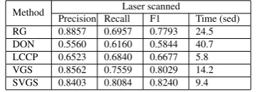
the details of a complete structure are segmented as individual parts. In contrast, the result of SVGS method is more like the under-segmented one, which prefers to keep the large object as a complete segment, for example, the neighboring surfaces of the same facade are recognized as one planar surface. It is also noteworthy that in the result of SVGS, many small details are merged as larger objects and preserved in the output, for example, the window frames. However, for that of VGS, the over-segmented objects consisting of merely one voxel are removed as outliers from the output. Of cause, this is counterproductive to the completeness of the output results. To carry out a quantitative evaluation, we compare our methods with reference methods using the manually segmented ground truth data, consisting of 33 segments. Here, the voxel resolution used in VGS, SVGS, and LCCP is 0.1 m, equaling to the radius of normal vecotr estimation in RG and the small radius of normal estimation in DON. The seed resolution of supervoxel in SVGS and LCCP is 0.2 m, equaling to the graph size used in VGS and the large radius of normal estimation in DON. The graph size of SVGS is 0.4 m. As shown in Table 1, our proposed methods can outperform other reference methods according to the F1 scores, with the value reaching around 0.81. It is noteworthy that the result of RG method is comparable with those of our methods, but when it comes to the execution time, our methods are more efficient.
Method Laser scanned
Precision Recall F1 Time (sed)
RG 0.8857 0.6957 0.7793 24.5
DON 0.5560 0.6160 0.5844 40.7
LCCP 0.6523 0.6840 0.6677 5.8
VGS 0.8562 0.7559 0.8029 14.2
SVGS 0.8403 0.8084 0.8240 9.4
Table 1. Evaluation of segmentation results of the building facade dataset
5.3 Results of construction site scene
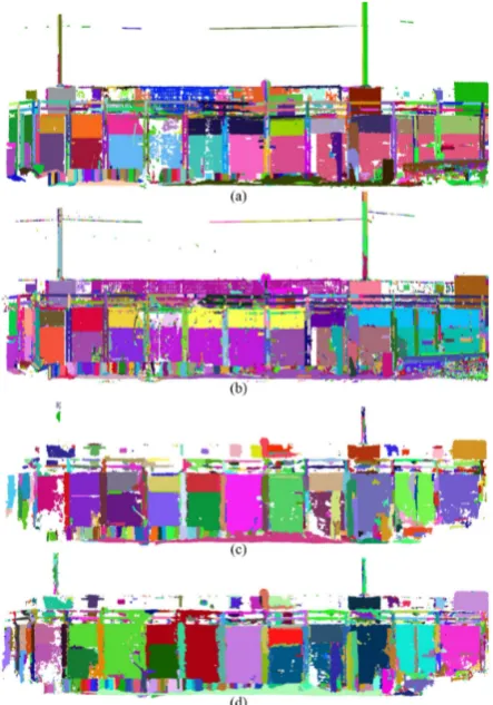
For the test in the scene of construction site, segmentation re-sults of point clouds generated by LiDAR and photogrammetry are illustrated in Fig. 8, with VGS and SVGS methods used. Similarly, different segments are rendered with varying colors. The parameters of methods are same as the ones used for the case of building facade. It appears that, the environments of the construction site scene is much more complex than that of the building facade, which significantly increases the difficulties of segmentation. This can also be proved from the results, which are obviously inferior to the result of building facade case. Com-paring the results of using LiDAR and photogrammetric datasets, we can easily find that, for segmenting the major structures of the ISPRS Annals of the Photogrammetry, Remote Sensing and Spatial Information Sciences, Volume IV-1/W1, 2017
Figure 7. Segmentation of building facade using (a) VGS and (b) SVGS methods.
given point clouds, the result of using LiDAR data is much better than that of using photogrammetry. One of the possible reason is that, unlike the LiDAR points, the positions of photogrammetric points normally have larger errors due to the stereo matching process, which may decrease the accuracy of spatial positions of these points. Moreover, the VGS method shows better per-formance using photogrammetric dataset, when compared with that of SVGS methods, especially in the preservation of concave and “stair-like” connections. This is because for the SVGS method, the generation of supervoxels are sensitive to the higher percentage of noise and outliers existing in the photogrammetric dataset, as they are clustered by the use of normal vectors.
For the quantitative evaluation, as listed in the Table. 2, our VGS and SVGS methods can outperform the other methods, withF1 - scores larger than 0.7, for both LiDAR and photogrammetric datasets. Interestingly, for the testing sample point cloud, the testing results of photogrammetric datasets are even better than those using LiDAR ones, for both VGS and SVGS methods, according to theF1- scores. One of the possible explanation for this phenomenon is due to the ground truth we used. Since the manually segmented ground truth of photogrammetric dataset is rougher than that of LiDAR dataset, it may influence the correcte-ness of the evaluation. For the photogrammetric dataset we used, it is difficult to manually segment the point cloud even for our human vision because of its quality. This phenomenon can also be observed from the results comparisons of using other reference methods. Therefore, in our future work, for providing more convincing evaluation results, a reliable ground truth is necessary. But then again, although the comparison using different ground truth datasets is not appropriate, the evaluation using the same ground truth can still support the superior performance of our proposed methods.
Method Laser scanned Photogrammetric
Precision Recall F1 Precision Recall F1
RG 0.6098 0.5799 0.5945 0.6371 0.6807 0.6582
DON 0.5875 0.5160 0.5495 0.5649 0.5269 0.5452 LCCP 0.5950 0.5250 0.5578 0.6104 0.5694 0.5892 VGS 0.7105 0.7077 0.7091 0.7655 0.7306 0.7476 SVGS 0.7205 0.7283 0.7244 0.7163 0.7420 0.7289
Table 2. Evaluation results of the construction site dataset
6. CONCLUSION
In this paper, we report a strategy for point cloud segmentation, using voxel structure and graph-based clustering with perceptual laws, which allows a learning-free and completely automatic but parametric method for segmenting 3D point cloud. The
Figure 8. Segmentation results of construction site using (a) VGS and (b) SVGS methods with LiDAR dataset, and using (c)
VGS and (d) SVGS methods with photogrammetric dataset.
experiments using different datasets have demonstrated that our proposed methods can achieve segmentation results effectively and efficiently, especially for complex scenes and nonplanar sur-faces of objects. In addition, quantitative comparisons between our method and other representative segmentation methods also validate the superior performance of our methods.
REFERENCES
Aldoma, A., Marton, Z.-C., Tombari, F., Wohlkinger, W., Pot-thast, C., Zeisl, B., Rusu, R. B., Gedikli, S. and Vincze, M., 2012. Point cloud library.IEEE Robotics & Automation Magazine.
Awrangjeb, M. and Fraser, C. S., 2014. Automatic segmentation of raw lidar data for extraction of building roofs.Remote Sensing 6(5), pp. 3716–3751.
Ballard, D. H., 1981. Generalizing the hough transform to detect arbitrary shapes.Pattern recognition13(2), pp. 111–122.
Besl, P. J. and Jain, R. C., 1988. Segmentation through variable-order surface fitting. IEEE Transactions on Pattern Analysis and Machine Intelligence10(2), pp. 167–192.
Comaniciu, D. and Meer, P., 2002. Mean shift: A robust approach toward feature space analysis. IEEE Transactions on pattern analysis and machine intelligence24(5), pp. 603–619.
Felzenszwalb, P. F. and Huttenlocher, D. P., 2004. Efficient graph-based image segmentation. International Journal of Com-puter Vision59(2), pp. 167–181.
Golovinskiy, A. and Funkhouser, T., 2009. Min-cut based segmentation of point clouds. In: Computer Vision Workshops (ICCV Workshops), 2009 IEEE 12th International Conference on, IEEE, pp. 39–46.
Green, W. R. and Grobler, H., 2015. Normal distribution trans-form graph-based point cloud segmentation. In:Pattern Recog-nition Association of South Africa and Robotics and Mechatron-ics International Conference (PRASA-RobMech), 2015, IEEE, pp. 54–59.
Hackel, T., Wegner, J. D. and Schindler, K., 2016a. Contour detection in unstructured 3d point clouds. In:Proceedings of the IEEE Conference on Computer Vision and Pattern Recognition, pp. 1610–1618.
Hackel, T., Wegner, J. D. and Schindler, K., 2016b. Fast semantic segmentation of 3d point clouds with strongly varying density. IS-PRS Annals of the Photogrammetry, Remote Sensing and Spatial Information Sciences, Prague, Czech Republic3, pp. 177–184.
Ioannou, Y., Taati, B., Harrap, R. and Greenspan, M., 2012. Difference of normals as a multi-scale operator in unorganized point clouds. In: Proceedings of the 2012 Second International Conference on 3D Imaging, Modeling, Processing, Visualization & Transmission, 3DIMPVT ’12, IEEE Computer Society, Wash-ington, DC, USA, pp. 501–508.
Morsdorf, F., Meier, E., Allg¨ower, B. and N¨uesch, D., 2003. Clustering in airborne laser scanning raw data for segmentation of single trees. International Archives of the Photogrammetry, Remote Sensing and Spatial Information Sciences 34(part 3), pp. W13.
Nurunnabi, A., Belton, D. and West, G., 2012. Robust segmenta-tion for multiple planar surface extracsegmenta-tion in laser scanning 3d point cloud data. In: Pattern Recognition (ICPR), 2012 21st International Conference on, IEEE, pp. 1367–1370.
Papon, J., Abramov, A., Schoeler, M. and Worgotter, F., 2013. Voxel cloud connectivity segmentation-supervoxels for point clouds. In: Proceedings of the IEEE Conference on Computer Vision and Pattern Recognition, pp. 2027–2034.
Peng, B., Zhang, L. and Zhang, D., 2013. A survey of graph the-oretical approaches to image segmentation. Pattern Recognition 46(3), pp. 1020–1038.
Pham, T. T., Eich, M., Reid, I. and Wyeth, G., 2016. Geo-metrically consistent plane extraction for dense indoor 3d maps segmentation. In: Intelligent Robots and Systems (IROS), 2016 IEEE/RSJ International Conference on, IEEE, pp. 4199–4204.
Rabbani, T., Van Den Heuvel, F. and Vosselmann, G., 2006. Segmentation of point clouds using smoothness constraint. Int. Arch. Photogramm. Remote Sens. Spatial Inf. Sci.36(5), pp. 248– 253.
Ramiya, A. M., Nidamanuri, R. R. and Ramakrishnan, K., 2016. A supervoxel-based spectro-spatial approach for 3d urban point cloud labelling.International Journal of Remote Sensing37(17), pp. 4172–4200.
Richtsfeld, A., M¨orwald, T., Prankl, J., Zillich, M. and Vincze, M., 2014. Learning of perceptual grouping for object segmenta-tion on rgb-d data. Journal of visual communication and image representation25(1), pp. 64–73.
Rusu, R. B. and Cousins, S., 2011. 3d is here: Point cloud library (pcl). In: Robotics and Automation (ICRA), 2011 IEEE International Conference on, IEEE, pp. 1–4.
Rusu, R. B., Blodow, N., Marton, Z. C. and Beetz, M., 2009. Close-range scene segmentation and reconstruction of 3d point cloud maps for mobile manipulation in domestic environments. In: 2009 IEEE/RSJ International Conference on Intelligent Robots and Systems, IEEE, pp. 1–6.
Salti, S., Tombari, F. and Di Stefano, L., 2014. Shot: unique signatures of histograms for surface and texture description. Comput.Vis. Imag. Understanding125, pp. 251–264.
Schnabel, R., Wahl, R. and Klein, R., 2007. Efficient ransac for point-cloud shape detection. In: Computer graphics forum, Vol. 26number 2, Wiley Online Library, pp. 214–226.
Stein, S., Schoeler, M., Papon, J. and Worgotter, F., 2014. Ob-ject partitioning using local convexity. In: Proceedings of the IEEE Conference on Computer Vision and Pattern Recognition, pp. 304–311.
Su, Y.-T., Bethel, J. and Hu, S., 2016. Octree-based segmentation for terrestrial lidar point cloud data in industrial applications. ISPRS Journal of Photogrammetry and Remote Sensing 113, pp. 59–74.
T´ov´ari, D. and Pfeifer, N., 2005. Segmentation based robust interpolation-a new approach to laser data filtering.International Archives of Photogrammetry, Remote Sensing and Spatial Infor-mation Sciences36(3/W19), pp. 79–84.
Tuttas, S., Braun, A., Borrmann, A. and Stilla, U., 2014. Com-parision of photogrammetric point clouds with bim building el-ements for construction progress monitoring. The International Archives of Photogrammetry, Remote Sensing and Spatial Infor-mation Sciences40(3), pp. 341.
Vo, A.-V., Truong-Hong, L., Laefer, D. F. and Bertolotto, M., 2015. Octree-based region growing for point cloud segmentation. ISPRS Journal of Photogrammetry and Remote Sensing 104, pp. 88–100.
Vosselman, G., 2013. Point cloud segmentation for urban scene classification.ISPRS Int. Arch. Photogramm. Remote Sens. Spat. Inf. Sci.
Vosselman, G. and Maas, H.-G., 2010. Airborne and terrestrial laser scanning. Whittles Publishing.
Vosselman, G., Gorte, B. G., Sithole, G. and Rabbani, T., 2004. Recognising structure in laser scanner point clouds.International archives of photogrammetry, remote sensing and spatial informa-tion sciences46(8), pp. 33–38.
Wang, M. and Tseng, Y.-H., 2011. Incremental segmentation of lidar point clouds with an octree-structured voxel space. The Photogrammetric Record26(133), pp. 32–57.
Weinmann, M., Jutzi, B., Hinz, S. and Mallet, C., 2015. Seman-tic point cloud interpretation based on optimal neighborhoods, relevant features and efficient classifiers. ISPRS Journal of Photogrammetry and Remote Sensing105, pp. 286–304.
Xu, Y., Tuttas, S. and Stilla, U., 2016. Segmentation of 3d outdoor scenes using hierarchical clustering structure and per-ceptual grouping laws. In:2016 9th IAPR Workshop on Pattern Recogniton in Remote Sensing (PRRS), pp. 1–6.
Xu, Y., Tuttas, S., Hoegner, L. and Stilla, U., 2017. Geometric primitive extraction from point clouds of construction sites us-ing vgs. IEEE Geoscience and Remote Sensing Letters14(3), pp. 424–428.