CONTRIBUTION OF MODIS SATELLITE IMAGE TO ESTIMATE THE DAILY AIR
TEMPERATURE IN THE CASABLANCA CITY, MOROCCO
Hicham Bahi *a, Hassan Rhinane a, Ahmed Bensalmia a
a
Faculty of Sciences Ain Chock, University Hassan II, Casablanca, Morocco - (bahi.h88, h.rhinane)@gmail.com, [email protected]
KEY WORDS: Air temperature, land surface temperature, LST, MODIS, Casablanca, remote sensing, urban climate.
ABSTRACT:
Air temperature is considered to be an essential variable for the study and analysis of meteorological regimes and chronics. However, the implementation of a daily monitoring of this variable is very difficult to achieve. It requires sufficient of measurements stations density, meteorological parks and favourable logistics. The present work aims to establish relationship between day and night land surface temperatures from MODIS data and the daily measurements of air temperature acquired between [2011-20112] and provided by the Department of National Meteorology [DMN] of Casablanca, Morocco. The results of the statistical analysis show significant interdependence during night observations with correlation coefficient of R²=0.921 and Root Mean Square Error RMSE=1.503 for Tmin while the physical magnitude estimated from daytime MODIS observation shows a relatively coarse error with R²=0.775 and RMSE=2.037 for Tmax. A method based on Gaussian process regression was applied to compute the spatial distribution of air temperature from MODIS throughout the city of Casablanca.
1. INTRODUCTION
The temperature of the urban air canopy represents an important element in the regional climate. However, owing to the heterogeneity bound up with numerous environmental factors that regulate the energy balance of the land-atmosphere system, such as vegetation coverage and albedo, the spatial patterns of air temperature can be highly variable and complex (Benali et al., 2012). Considering that the physical magnitude, air temperature, measured by the meteorological stations supply only limited information about spatial patterns over a wide area, the technique of remote sensing remains an appropriate and a promising technology to provide a more precise description of the spatial distribution of air temperature on both regional and global scales (Sun et al., 2013).
The spatial distribution of air temperature remains a suitable environmental variable because it can be used as an input data in numerous applications in the ecological fields. So it will be useful to monitor evapo-transpiration and simulate the performance of potential crops in order to assess food security, to study the propagation and transmission of diseases, such as the case of influenza virus (Lowen et al., 2007), or to assess the risks of climate change (Solomon et al., 2007). The traditional method that allows us to determine the spatial variation of air temperature is often based on a spatial interpolation and extrapolation of data from the nearest weather stations. This technique remains the mostly used one, and makes use of a statistical algorithm called Kriging with external drift (Hudson and Wackernagel, 1994). This is an estimator including widely sampled secondary data to characterize the spatial pattern of this variable. The problem with the interpolation and extrapolation of air temperature is that they depend on many local parameters which may influence the estimation of the spatial distribution of air temperature such as altitude, sun exposure, terrain concavity and distance from the coast (Marquínez et al., 2003).
The land surface temperature (LST) is one of the essential parameters for the estimation of this quantity. According to
(Vancutsem et al., 2010), the difference between the temperature of the surface derived from daytime MODIS (Moderate Resolution Imaging Spectro-radiometer) product and the maximum temperature vary significantly by region and season, while the nighttime MODIS observation ensures a better estimation of the minimum air temperature in different regions in Africa (Vancutsem et al., 2010). As an appendix, Méndez has mentioned that the temperature of the area decreases when the altitude at the sea level increases, and proposed a method to evaluate the temperature of the air depending on the elevation of each pixel and its proper pressure (Méndez, 2004). Others have shown that the temperature (freshness-based areas) depends significantly on the abundance of vegetation (Rhinane et al., 2012), and this quantity can be expressed by an extrapolation of the NDVI (Normalized Difference Vegetation Index) during the seasons of winter, spring and summer while the strength of the relationship remains insignificant in the autumn period (Sun and Kafatos, 2007).
The main purpose of this study is to use the techniques of remote sensing to investigate the spatial distribution of daily minimum, average and maximum air temperature using MODIS observation (MOD11A1 product) over the city of Casablanca by developing a model based on a statistical approach. The accuracy of the air temperature estimated has been investigated by validating the results against the data from measurement station.
The choice of the city of Casablanca is strategic for our study because it is considered among the important cities affected by micro urban heat islands and also by increases of ambient temperature (Rhinane et al., 2012). Apart its coastal location, population density and the urban development of the city, Casablanca is considered as the most productive city in Morocco, theses industrial and commercial activities make it vulnerable to climate warming. Indeed, the average temperature has increased during the period 1961-2008, with a trend of 0.3°C per decade (Rhinane et al., 2012; World Bank and CMI, 2011), about the future projection for 2030 the economic The International Archives of the Photogrammetry, Remote Sensing and Spatial Information Sciences, Volume XLII-2/W1, 2016
metropolis foresee a warming of 1.3 °C, accompanied by a agglomeration which is spread over an area of 386 km ², hence the need to estimate the spatial distribution of the air temperature in this economic metropolis.
2. STUDY AREA AND DATA 2.1 Study area
The city of Casablanca, the economic capital of the country and one of the largest metropolises in the continent, is located in the Central West of Morocco spread over Chawiya plains (Lat 33 ° 36'N, Long 07 ° 36'W) (Figure 1), with altitude that varies between 0 and 163 m. the Casablanca city cover over an area of 386 Km² with population of approximately 4 million inhabitants.
Figure 1. Study area
Its geographical location at the edge of the Atlantic Ocean gives it an oceanic climate with a mild and rainy winter, and a humid and temperate summer without precipitation. The average annual temperature is 18.88 °C, with a minimum temperature of 7°C and maximum of 27°C. In term of rainfall, the annual total of precipitation varies considerably. The economic metropolis knows high humidity throughout the year with absence of frost in winter.
2.2 Data
2.2.1 Satellite data
The MODIS observations are an important source for the study of the climate, vegetation, pollution, and various meteorological phenomena. They are stored in a hierarchical data format (HDF) to facilitate the sharing of this scientific data in different platforms.
In order to estimate the daily air temperature we use MOD11A1 product for a series of years ranging from 2011 to 2012. The MODIS LST images used are projected on sinusoidal grid with a resolution of 1 km (exactly 0.927 km), and were derived from the two thermal infrared bands, band 31 (10.78-11.28 µm) and 32 (11.77-12.27 µm), using the "Split-Window" algorithm. This algorithm permits to correct the atmospheric action and different effects of emissivity (Wan, 2007; Wan, 1999). The HDF file of MOD11A1 product comprises the following Science Data Set (SDS): layers for day time and night time observations LSTs, quality control assessments, observation times, view zenith angles, clear sky coverage, and bands 31 and
32 of emissivity from land cover types (Wan, 2007). In this study we will look at the both local attributes LST_Day_1km and LST_Night_1km that refer respectively to the diurnal and nocturnal land surface temperature.
Several studies have shown that the accuracy of the MODIS LST product is less than 1°C in the absence of cloud cover, and errors can occur due to large uncertainties in the emissivity of
The meteorological data used, minimum, average and maximum air temperature were provided by the Department of the National Meteorology (DMN) and were generated by thermometers installed in shelters louvered with double roof at height of 2m above the ground. Minimum temperatures were acquired by alcohol thermometers while maximum temperatures were acquired by mercury thermometers (Table 1).
Name of station Latitude Longitude Altitude
Casa-wilaya 33.59 -7.62 25 m
Table 1. Geographical references of the measuring station.
3. METHODOLOGY
The figure 2 summarize the methodology adopted in this paper.
Figure 2. The processing used for estimating the daily air temperature
3.1 Determining the number of cloudless day
Although MODIS sensors provide daily images, these are not continuous due to abundant presence of clouds. In fact, the Casablanca region weather is characterized by a sky sometimes cloudy and sometimes clear with a light breeze, which explains the lack of information of LST during consecutive days. The abundance of clouds depends on the yearly seasons. During winter, it is much more conducive to clouds than the summer period. It is also possible that MODIS temperatures measurement will be colder than the real LST, this is due mainly to the difficulty of distinguishing thin clouds as the case of cirrus (Timothy et al., 2002).
The amount of clouds present over a year can be assessed by calculating the ratio between the numbers of days with effective The International Archives of the Photogrammetry, Remote Sensing and Spatial Information Sciences, Volume XLII-2/W1, 2016
measures of LST on the number of days in a year. Thus, in the Casablanca region approximately 60.1% of days allowed measures of daytime LST during the two years 2011 and 2012, against 60.8% for nighttime LST (table 2).
2011 2012 Average over the two years (2011-2012)
LST_DAY 56,44 % 64,38 % 60,1 %
LST_NIGHT 58,63 % 63,29 % 60,8 % Table 2. Percentage of the number of cloudless days of the MODIS Terra product during the two years 2011 and 2012
All values used in this study are values which refer to cloudless days.
3.2 Estimation of the air temperature
The evaluation of the physical magnitude deduced, air temperature, is based on a statistical approach. In this approach we will compare the local attributes LST_NIGHT and LST_DAY of MOD11A1 product with the meteorological observations Tmin, Tmax and Tavg using regression analysis, in order to deduce the linear, quadratic, cubic or exponential function that binds these two quantities (Equations 1 to 4). The correlation between nighttime / daytime LST and air temperature was investigated by calculating the correlation coefficient of Pearson product-moment (Equation 5).
= × + (1)
Where R = Correlation coefficient Ta = Air temperature
Tai = Air temperature measured by the
meteorological station in the i-th day Ta = Arithmetic average of air temperature
LST = Daytime/nighttime land surface temperature of the MOD11A1 product
LSTi = Land surface temperature of the MOD11A1 product in the i-th day
= Arithmetic average of LSTi
a, b ,c and d are parameters that varies according to the model selected (table 3).
In order to achieve a more satisfactory fit several models based on a statistical approach have been established, among these models (table 3):
Model 1: Comparison with nighttime observations.
Model 2: Comparison with daytime observations.
Model 3: Correlation with average day and night.
Model 4: Comparison with winter periods.
Model 5: Comparison with summer periods.
Model 6: Multiple correlation between Ta, LST and day length.
3.3 Interpolation of spatial distribution of Ta
Many studies have shown that the air temperature decreases with altitude at approximately 6.5 °C per Km (Rolland, 2003). Therefore the interpolation method should be preceded by critical step which consists of making relationship between temperature and elevation in order to compensate the altitude
effect (willmott and Matsuura, 1995). In this study we apply interpolation method called Universal Kriging plus the Digital Elevation Model correction (UnK+DEM method) mentioned in (Nguyen et al., 2015). The Gaussian process regression (also called Kriging) applied after Elevation Correction for Temperature (ECT) allow us to gives the best linear unbiased evaluated from MODIS observations and the air temperature supplied by the measurement stations. The most widely used indicator to evaluate the interest of predictive values is the
RMSE (Root Mean Square Error also called “RMSD” Root
Mean Squared Deviation). This indicator represents the mean deviation between any simulated values and their equivalent measured. The root mean square error is written as follows:
= 1 (� − �)2
=1 (6)
Where N = number of observations
� = estimated value (prediction value)
� = measured value
The other indicator used in this research to evaluate the model is the MAE (Mean Absolute Error), which is less affected by the most important prediction errors (willmott and Matsuura, 2005).
� =1 � − � =1 (7)
4. RESULTS AND DISCUSSION
The relationship between the daily air temperature and MODIS LST observations was determined by regression analysis during time series ranging from 2011 to 2012. In this study, several models have been established in order to achieve more fit satisfactory but only 6 models, whose residues do not mark a big gap, were selected (table 3).
All the indices in (table 3) show that the interdependence between the calculated and predicted air temperature are significant with a tolerable average absolute error ranging from 0.844 to 1.376°C and a mean square error that does not exceed 2.103°C. The analysis of these models indicates that the nighttime MODIS LST observations provide a better estimation of daily air temperature with R² contained in the interval [0.824; 0.921] and RMSE contained in the interval [1.332; 1.810] (Model 1) against R² contained in the interval [0.773; 0.891] and RMSE contained in the interval [1.526; 2.038] for daytime MODIS observations (model 2). The results also show that during the year the average temperature expressed from the local attribute LST_NIGHT of the MOD11A1 product, according to the model 1, remains the most important predictor with a correlation coefficient of R² ≥ 0.918 and RMSE ≤ 1.338°C.
The decreasing of the air temperature error estimated from nighttime MODIS observations can be explained by anthropogenic causes promoting the emergence of air pollution are reduced overnight. Indeed, the pollution caused by vehicle exhausts becomes futile overnight because the traffic is almost nil during this period. Similarly for hazardous pollutants generated by industrial activities that occur in a rational manner during the night periods. However gaseous emissions such as nitrogen oxide and sulphur dioxide reach their peak during the day and contribute to the increase of atmospheric effects. The interaction of the radiation with the anthropogenic aerosols The International Archives of the Photogrammetry, Remote Sensing and Spatial Information Sciences, Volume XLII-2/W1, 2016
previously mentioned causes errors in estimating emissivity (Timothy et al., 2002), and therefore causes indirect disturbances on the calculation of the near surface temperature
by different methods (Corwin and Rodenburghii, 1994), which explains the increase of errors in the model 2.
Equation Tmin Tmax Tavg
R2 RMSE MAE R2 RMSE MAE R2 RMSE MAE
Model 1: Comparison with nighttime observations
× + 0.920 1.511 1.167 0.826 1.796 1.208 0.919 1.332 0.926
× + × ( )2+ × ( )3+ 0.921 1.503 1.157 0.829 1.780 1.210 0.918 1.338 0.929
b × e(a ln (LSTnight)) 0.907 1.623 1.255 0.824 1.810 1.193 0.919 1.336 0.921
Model 2: Comparison with daytime observations
× �+ 0.905 1.617 1.215 0.773 2.045 1.376 0.889 1.538 1.079
× �+ × ( �)2+ 0.908 1.594 1.201 0.775 2.037 1.360 0.891 1.526 1.069
b × e(a ln (LSTday)) 0.905 1.621 1.218 0.775 2.038 1.366 0.889 1.535 1.077
Model 3: Correlation with average day and night
× ( �+ )/2 + 0.905 1.651 1.261 0.803 1.886 1.220 0.893 1.526 1.058
× � + × ( � )2+ × (
� )3+ 0.907 1.631 1.238 0.804 1.886 1.224 0.912 1.388 0.969
b × e(a ×ln (LSTavg)) || b × e(a × LSTavg) 0.904 1.656 1.265 0.803 1.888 1.238 0.910 1.405 0.960
Model 4: Comparison with winter periods
× + 0.863 1.570 1.221 0.768 1.739 1.181 0.876 1.323 0.931
× + × ( )2+ × ( )3+ 0.859 1.558 1.245 0.784 1.678 1.139 0.879 1.304 0.920
b × e(a×ln (LSTday)) || b × e(a × LSTday) 0.863 1.571 1.221 0.778 1.699 1.151 0.880 1.299 0.915
Model 5: Comparison with summer periods
× + 0.312 1.172 0.858 0.206 2.041 1.222 0.276 1.438 0.920
× + × ( )2+ × ( )3+ 0.337 1.151 0.844 0.152 2.103 1.197 0.401 1.314 0.888
b × e(a ×ln (LSTday)) || b × e(a × LSTday) 0.316 1.169 0.856 0.152 2.103 1.197 0.290 1.424 0.922
Model 6: Multiple correlation between Ta, LST and day length
× + × �+ × + 0.910 1.603 1.202 0.819 1.815 1.183 0.915 1.363 0.945
× + × �+ × +
× × �− + × cos �× + 0.914 1.572 1.182 0.812 1.838 1.214 0.918 1.346 0.949
Table 3. Model equations and accuracy validation of minimum, average and maximum air temperature (a, b, c, d, f and g are parameters; SD: Sunshine Duration; LSTavg: average between LSTday and LSTnight)
Another factor explaining the increasing of estimation errors during the daytime is the atmospheric turbulence which plays a decisive role in the quality of the image (Shimizu et al., 2008). Several studies have shown that stratification in the distribution of layers also depends on the time of observation.
During day-times, there is a substantial turbulence on the ground because of heating localized in the soil in addition to the effect of wind shear, while at night the turbulence is shown in altitude (Rocca et al., 1974). Since it is a temperature inversion in the lower atmosphere (the ground cools faster than the air), hot air stagnates above the cold air masses, creating stability in the lower atmosphere (Khare and Sharma, 1999). Thus, to minimize the prediction errors due to different atmospheric effects, it is more suitable to estimate the air temperature only from nighttime MODIS observations (Model 4 and 5).
The model 3 accentuates what has previously been affirmed, and shows that by combining and adding local attributes LST_DAY, which are most affected by atmospheric effects, with nighttime MODIS observations, prediction errors become relatively important.
Figure 3. Correlation graph between Daytime MODIS LST and Tmax.
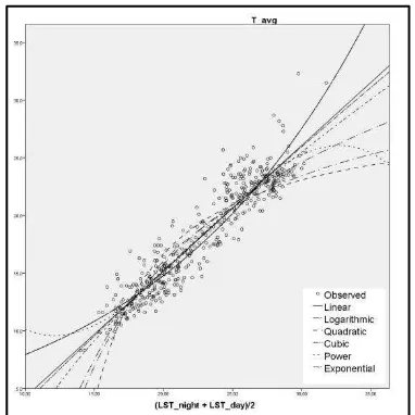
Figure 4. Correlation graph between Tavg and the average of Daytime and nighttime MODIS LST.
Figure 5. Correlation between nighttime MODIS LST and Tmin
The graphs (figure 3,4 and 5) represent the linear, quadratic, cubic and exponential function that allow us to bind the air temperature calculated by the measurement station and LST. And as mentioned in the previous paragraph, it can be deduced from the (figure 8) that the nighttime MODIS observations allowed a better estimation of minimum air temperature. While in the estimation of maximum air temperature (figure 6) from daytime MODIS observations, we had four exceedances of confidence intervals (exceedances of UCL: Upper Control Limit) during the two years 2011 and 2012. These exceedances it can be due mainly to different atmospheric effects or to difficulty of distinguishing the thin cloud as the case of cirrus (Liu et al., 2004). The same result is shown for average air temperature estimated from the mean of daytime and nighttime MODIS observations (figure 7).
Figure 6. Time series curve of Tmax from 2011 to 2012 (UCL: Upper Control Limit; LCL: Lower Control Limit).
Figure 7. Time series curve of Tavg from 2011 to 2012 (UCL: Upper Control Limit; LCL: Lower Control Limit).
Figure 8. Time series curve of Tmin from 2011 to 2012 (UCL: Upper Control Limit; LCL: Lower Control Limit).
In order to better understand the assessment of air temperature during a yearly period we divided the raster and meteorological data into two parts, for each parts the statistical analysis was performed separately. The first part, dated from October 1st to 31 May, referring to the winter season (including intermediate seasons) (model 4), while the second part, which dates from June 1st to September 31, refers to the summer season (model 5).
The results show that the cubic function applied on the data from the first part, during the winter period, allows better quantifying of the average and maximum temperatures with mean absolute errors of 0.920 and 1.139°C, respectively, and a mean square error of 1.304°C for Tavg and 1.678 for Tmax. On the other hand, we find that quantifying the strength of the relationship between the minimum temperature and the nighttime MODIS observation is more beneficial during the summer (model 5) with MAE ≤ 0.858°C and RMSE ≤ 1.172°C. The presence of a relatively low coefficient of correlation in Model 5 does not compromise the obtained results. Indeed, the results in (Table 4) shows that the correlation coefficient The International Archives of the Photogrammetry, Remote Sensing and Spatial Information Sciences, Volume XLII-2/W1, 2016
between the physical quantity deducted and calculated is significant at 0.001 for linear function and 0.00 for the cubic and power function, which proves that the association is confirmed and the estimation errors calculated, namely RMSE and MAE, are far from being obtained by a simple chance. The addition of a marginal variable, sunshine duration, as a weighting variable in model 6 allowed us to better calibrate model 3. Indeed, the error of the deduced average temperature expressed in terms of two local attributes LST_DAY and LST_NIGHT was slightly lower in the model 6 with a reduction rate of order 1.58% compared to model 3.
Correlation F(LST_Night)
linear
F(LST_Night) cubic
F(LST_Night) power
R2 Pearson .312** .337** .316**
Sig. (bilateral) .001 .000 .000
N 150 150 150
**. The correlation is significant at the 0.01 level (bilateral). Table 4. Significance test of R Pearson
The marginal variable, sunshine duration, was calculated by using the following formula (Rezoug and Zaatri, 2011):
= 2 ×� (−tan�× tan�) ×12
� (8)
�= 23.45 × sin(2π284+n
365 ) (9)
Where SD = sunshine duration
= Parallel of latitude β
n = date (n days after the spring equinox)
= angle described by the Earth on its orbit for n days
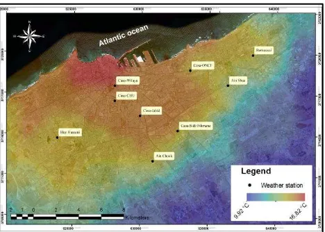
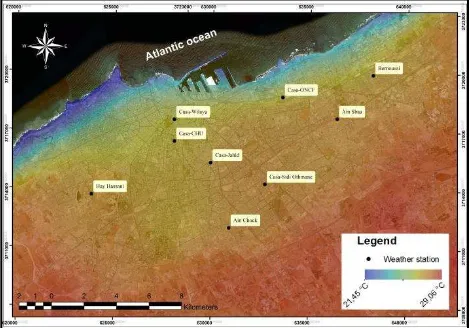
After treatment and processing of the satellite images, we obtain the following maps (figure 9, 10, 11, 12 & 13) that provide the spatial distribution of minimum and maximum air temperature estimated from nighttime and daytime MODIS observation during the 4th of February, 19th of March, 3th of August, 7th of August and 18th of December 2012. The results show that during the summer periods and during the daytime the minimum temperatures are marked in coastal areas, and then the temperature rises gradually towards the center, as the case of the region of Ain Chock and Sidi Moumen, with emergence of high temperatures in a more intense manner in remote areas and in the suburban of Casablanca (figure 13). During the winter periods, the high temperatures are coinciding with heat islands of the layer of urban air canopy. And unlike to the summer period, the high temperatures are marked even more significantly inside the city as the case of the areas covered by dense built (tinted areas in yellow) and the industrial areas of Ain Sebaâ and Roche Noire (tinted areas in red) experiencing a significant release of air pollution (Rhinane et al., 2012) (figure12). During the night, the spatial representations of the minimum air temperature are distributed in the same manner during all the year with the concentration of the heat island of urban air canopy in the center of the city (figure 9, 10 & 11).
Figure 9. Spatial distribution of minimum air temperature estimated from nighttime MODIS observation during the 19th
of March 2012
Figure 10. Spatial distribution of minimum air temperature estimated from nighttime MODIS observation during the 3th of
august 2012
Figure 11. Spatial distribution of minimum air temperature estimated from nighttime MODIS observation during the 18th
of December 2012
Figure 12. Spatial distribution of maximum air temperature estimated from daytime MODIS observation during the 4th of
February 2012
Figure 13. Spatial distribution of maximum air temperature estimated from daytime MODIS observation during the 7th of
August 2012
Our results show also that the UnK+DEM interpolation results are consistently better with surface observations than traditional interpolation methods and produce a better visual effect than the original images.
In this study the results of the statistical approach for evaluation the spatial distribution of air temperature was performed by transferring the statistical relationships on all regions of Casablanca included the rural area. The lack of official weather stations in the neighbouring region can be responsible in a relative increase of the air temperature estimation errors in the rural municipalities. Consequently, the results evaluated according to the 9 measurement stations remain valid in the urban area of the Casablanca region and only for reference in the rest of the rural area.
Another factor that may affect the quality of the results obtained in the rural area of Casablanca region is the thermal properties of the soil and its open space which are completely different from the characteristics of an urban space. The measuring stations used for the validation of the results are located in urban area characterized by artificial surface, streets and elevated buildings. Therefore, this 3D geometry may undergo changes in the statistical relationships linking the physical quantity deduced and that calculated compared to the rural area, since it plays an important role in the variation of the air temperature in the space (Ren et al., 2008).
To resolve the problem relating to lack of weather stations and have good accuracy of spatial pattern of air temperature estimated in the rural municipalities not covered by the station measurement, several techniques can be established as the case of combining remote sensing and geographical predictors such as altitude, latitude, continentality and cloudiness factor (Ninyerola et al., 2000).
Several recent studies have highlighted what has previously been proved and have shown that the availability of some satellite data such as NOAA AVHRR or TERRA/ AQUA MODIS make it possible to combine the geographical approach with remote sensing data using variables related with air temperature such as LST, NDVI or albedo, and has been also shown that this technique makes it easier to reduce the errors (Cristobal et al., 2008).
Another approach may be beneficial to estimate the spatial distribution of the magnitude in question, and more specifically in rural areas and in vegetated urban areas. This method is based on the thermodynamics techniques which consists of using two parameters that are crop water stress index and aerodynamic resistance (Sun et al., 2005). Therefore, this technique allows to construct a quantitative relationship between the surface temperature and the ambient air temperature with an accuracy within 3°C in more than 80% of data processed (Sun et al., 2005).
5. CONCLUSION
The aim of the present paper is to evaluate the potential of daily MODIS LST as an indicator to estimate the spatial distribution of air temperature.
In this project we have highlighted the fact that it can be possible to estimate air temperature at height of 2 m above the ground from remotely sensed data. The suggested method allows us to solve the problem concerning the LST and air temperature by exploiting ground data of weather station measurement as reference. This interdependence between these two quantities, LST and Ta, was performed by correlation analysis and generalization of a set of equations.
The statistical approach followed in these models shows that all the correlations between the estimated and calculated variables are significant at 0.001 levels. And, the estimated air temperature remain a promising result since the obtained RMSE do not exceed approximately 2 °C, indeed, the cubic function of model 5 allow us better prediction of minimum and average air temperature with MAE of 0.844 and 0.888 °C respectively, while the exponential function of the model 4, provides a better estimation of maximum air temperature with MAE of 1.151°C. Regarding to the correlation coefficient, it shows a strong link between these two quantities, calculated and predicted air temperature, with R² equal to 0.921, 0.919 and 0.829 for Tmin, Tavg and Tmax respectively (model 1 of table 3).
The results show also that the strength of the link becomes more significant by separating data acquired in summer and winter periods in the statistical analysis or by adding other parameters as is the case with the sunshine duration.
The spatial distribution of air temperature estimated in this project and evaluated by the Gaussian interpolation method remains an appropriate environmental variable due to its use as input in different applications in environmental sciences, and it can, therefore, be useful in climate research and global change, controls many biological and physical processes between the hydrosphere, atmosphere and biosphere (Prihodko and Goward, 1997). This final result obtained, spatial representation of air temperature, it will be more promising if there were more station measurement in different municipalities of Casablanca region.
REFERENCES
Benali, A., Carvalho, A. C., Nunes, J. P., Carvalhais, N., & Santos, A., 2012. Estimating air surface temperature in Portugal using MODIS LST data. Remote Sensing of Environment, 124, pp. 108–121.
Coll, C., Wan, Z., & Galve, J. M., 2009. Temperature-based and radiance-based validations of the V5 MODIS land surface temperature product. Journal of Geophysical Research, 114, D20102. http://dx.doi.org/10.1029/2009JD012038.
Corwin, R. R., & Rodenburghii, A., 1994. Temperature error in radiation thermometry caused by emissivity and reflectance measurement error. Applied Optics, 33, pp. 1950-1957.
Cressie, N., 1990. The origins of kriging. Mathematical Building Energy Research, 5(1), pp. 7-41.
Hengeveld, H.G., 1990. Global Climate Change: Implications for Air Temperature and Water Supply in Canada. Transactions of the American Fisheries Society, 119(2), pp. 176-182.
Hudson, G., & Wackernagel, H., 1994. Mapping temperature using kriging with external drift – Theory and an example from Scotland. International Journal of Climatology, 14, pp. 77-91.
Jenerette, G.D., Harlan, S.L., Brazel, A., Jones, N., Larsen, L., & Stefanov, W.L., 2007. Regional relationships between surface temperature, vegetation, and human settlement in a rapidly urbanizing ecosystem. Landscape Ecology, 22(3), pp. 353-365.
Khare, M., & Sharma, P., 1999. Performance evaluation of general finite line source model for Delhi traffic conditions. Transportation Research Part D: Transport and Environment, 4, pp. 65-70.
Liu, Y., Key, J. R., Frey, R. A., Ackerman, S. A., & Menzel, P. W., 2004. Nighttime polar cloud detection with MODIS. Remote Sensing of Environment, 92(2), pp. 181–194.
Lowen, A. C., Mubareka, S., Steel, J., & Palese, P., 2007. Influenza virus transmission is dependent on relative humidity and temperature. PLoS Pathogens, 3, pp. 1470–1476.
Marquínez, J., Lastra, J., & García, P., 2003. Estimation models for precipitation in mountainous regions: The use of GIS and multivariate analysis. Journal of Hydrology, 270, pp.1-11.
Méndez, A. A., 2004. Estimate ambient air temperature at regional level using remote sensing techniques. MSc. Thesis. International Institute for GeoInformation Science and Earth Observation. temperature and appropriate resolution for satellite‐derived air temperature estimation. International Journal of Remote Sensing, 29:24, pp. 7213-7223.
Ninyerola, M., Pons, X., & Roure, J.M., 2000. A methodological approach of climatological modelling of air temperature and precipitation through GIS techniques. International Journal of Climatology, 20, pp. 1823–1841.
Prihodko, L., & Goward, S. N., 1997. Estimation of air temperature from remotely sensed surface observations. Remote Sensing of Environment, 60, pp. 335–346.
Ren, G., Zhou, Y., Chu, Z., Zhou, J., Zhang, A., Guo, J., & Liu, X., 2008. Urbanization Effects on Observed Surface Air Temperature Trends in North China. Journal of Climate, 21, pp. 1333–1348.
Rezoug, M. R., & Zaatri, A., 2011. Calcul de la durée optimale
d’activité d’un module photovoltaïque en fonction de l’endroit.
Revue des Energies Renouvelables, 14(1), pp. 163 - 169.
Rhinane, H., Hilali, A., Bahi, H., & Berrada, A., 2012. Contribution of Landsat TM data for the detection of urban heat islands areas case of Casablanca. Journal of Geographic Atmospheric Turbulent layers By Spatiotemporal and Sptioangular Correlation Measurements of Stellar light Scintillation. Journal of the Optical Society of America, 64, pp. 1000-1004.
Rolland, C., 2003. Spatial and seasonal variations of air temperature lapse rates in Alpine regions. Journal of Climate, 16, pp. 1032-1046.
Shimizu, M., Yoshimura, S., Tanaka, M., & Okutomi, M. (2008). Super-Resolution from Image Sequence under Influence of Hot-Air Optical Turbulence. Computer Vision and Pattern Recognition, 2008. CVPR 2008. IEEE Conference on, 1-8, doi: 10.1109/CVPR.2008.4587525.
Solomon, S., Qin, D., Manning, M., Chen, Z., Marquis, M., Averyt, K. B., Tignor, M., & Miller, H. L., 2007. Contribution of Working Group I to the Fourth Assessment Report of the Intergovernmental Panel on Climate Change. Cambridge University Press, Cambridge, United Kingdom and New York, USA., 996 pp.
Sun, D., & Kafatos, M., 2007. Note on the NDVI-LST relationship and the use of temperature-related drought indices over North America. Geophysical Research Letters, 34, L24406. http://dx.doi.org/10.1029/2007GL031485, 2007.
Sun, H., Chen, Y., Gong, A., Zhao, X., Zhan, W., & Wang, M., 2013. Estimating mean air temperature using MODIS day and The International Archives of the Photogrammetry, Remote Sensing and Spatial Information Sciences, Volume XLII-2/W1, 2016
night land surface temperatures. Theoretical and Applied Climatology, 118, pp. 81-92.
Sun, Y. J., Wang, J. F., Zhang, R. H., Gillies, R. R., Xue, Y., & Bo, Y. C., 2005. Air temperature retrieval from remote sensing data based on thermodynamics. Theoretical and Applied Climatology, 80, pp. 37-48.
Timothy, J. G., Lawrence, F. R., & Peter V. H., 2002. Aerosol Effects on Cloud Emissivity and Surface Longwave Heating in the Arctic. Journal of the Atmospheric Sciences, 59, pp. 769– 778.
Vancutsem, C., Ceccato, P., Dinku, T., & Connor, S. J., 2010. Evaluation of MODIS land surface temperature data estimate air temperature in different ecosystems over Africa. Remote Sensing of Environment, 114, pp. 449-465.
Wan, Z., 1999. MODIS Land-Surface Temperature. Algorithm Theoretical Basis Document. Accessed online in March 1 (2011). http://modis.gsfc.nasa.gov/data/atbd/atbd_mod11.pdf
Wan, Z., 2007. Collection-5, MODIS Land Surface Temperature Products Users' Guide, ICESS, University of
California, Santa Barbara.
http://www.icess.ucsb.edu/modis/LstUsrGuide/MODIS_LST_pr oducts_Users_guide_C5.pdf.
Wang, W., Liang, S., & Meyers, T., 2008. Validating MODIS land surface temperature products using long-term nighttime ground measurements. Remote Sensing of Environment, 112, pp. 623–35.
Weng, Q., Lub, D., & Schubringa, J., 2004. Estimation of land surface temperature–vegetation abundance relationship for urban heat island studies. Remote Sensing of Environment, 89(4), pp. 467–483.
Willmott, C. J., & Matsuura, K., 1995. Smart Interpolation of Annually Averaged Air Temperature in the United States. Journal of Applied Meteorology and Climatology, 34, pp. 2577–2586.
Willmott, C. J., & Matsuura, K., 2005. Advantages of the mean absolute error (MAE) over the root mean square error (RMSE) in assessing average model performance. CLIMATE RESEARCH, 30, pp. 79-82.
World Bank., the Marseille Center for Mediterranean Integration (CMI)., 2011. Adaptation au changement climatique
et aux désastres naturels des villes côtières d’Afrique du Nord.
Egis-BCEOM International; IAU îdF; BRGM, 2011.- 215 p. http://www.urbanknowledge.org/docs/coastal_cities.pdf
Xu, Y., Knudby, A., & Ho, H.C., 2014. Estimating daily maximum air temperature from MODIS in British Columbia, Canada. International Journal of Remote Sensing, 35(24), pp. 8108-8121.
Zhanga, W., Huanga, Y., Yua, Y., & Wenjuan Suna., 2011. Empirical models for estimating daily maximum, minimum and mean air temperatures with MODIS land surface temperatures. International Journal of Remote Sensing, 32(24), pp. 9415-9440.