A MULTIVARIATE ANALYSIS OF INDIVIDUAL,
SITUATIONAL AND ENVIRONMENTAL FACTORS
ASSOCIATED WITH POLICE ASSAULT INJURIES
Robert J. Kaminski
The State University of New York at Albany
David W. M. Sorensen
Rutgers University
Concern about police use of excessive force in the United States has increased over the last several years, due in part to the highly publicized videotaped beating of Rodney King by police in 1991 and the subsequent Los Angeles riot. Consequently, there has been a resurgence of interest in, and research on, police use of excessive force (e.g. Geller and Scott, 1992; Pate and Fridell, 1993a; Skolnick and Fyfe, 1993; Toch and Geller, 1995). However, there has been little recent research on violence against the police (but see Hirschel et al., 1994), and much of the previous work in this area has focussed on homicides of law enforcement officers (McLaughlin, 1992:22; Uchida and Brooks, 1988:1; Wilson and Meyer, 1990:32). While research on police use of excessive force and police homicides is important, there are several reasons for continued research on nonlethal police assaults.
death”; at the level of the police profession, assault victimization “hamper[s] the ability of agencies to recruit new officers; it can undermine police-community relations and it can threaten the professional image of practitioners”. Other research has shown that the threat of “physical attack on one’s person” and “situations requiring the use of force” are major job-related stressors in law enforcement work (Ellison and Genz, 1983; Speilberger et al., 1981). Furthermore, officers who have been attacked experience stress that can negatively affect their job performance in a variety of important ways (McMurray, 1990). Given such findings, it is not suprising that assaults on law enforcement officers are a major concern of government, police administrators and officers themselves (Hirschel et al., 1994: 115).
Rather than focussing on the etiology of police assaults per se, the current analysis examines factors that are associated with the likelihood of officer injury once an assault has taken place. While certain individual, situational, or environmental factors may increase or diminish the probability of police assaults, they do not necessarily correspond with those factors that increase or diminish the likelihood of injury. Enhanced knowledge regarding those factors associated with officer injury would thus prove useful for recruit training, and ultimately to departmental decision making. This study improves on much previous research by analyzing a broader spectrum of contributory factors, and by doing so within an appropriate multivariate context.
PREVIOUS RESEARCH ON POLICE ASSAULT
INJURIES
Prior research on police assault injuries can be divided into three methodological types, each representing an evolutionary improvement on the former. Many early studies employed simple cross-tabulations to identify relationships between variables and the likelihood of officer injury. Later research utilized “calls for service” base rates to control for exposure to harm. More recent and statistically sophisticated research has applied multiple regression techniques to the analysis of police assault injuries.
the research on police assault injuries has continued to focus on the probability of injury by type of call. Margarita (1980) cross-classified her assault data by injury and type of incident and found that injuries were most likely in the following circumstances: officer as victim (69.4%); other crimes (68.4%); public disturbances (64.9%); domestic disturbances (57.7%); mentally deranged persons (48.9%); and routine (47.5%) (Table 5-9, p. 133). Margarita also found that 97 percent of the officers seriously assaulted by assailants using personal weapons (i.e. hands, fist, feet) were injured (Figure 5-5, p. 130). Using bivariate analyses, Grennan (1987) examined the likelihood of injury in mixed-gender patrol teams and found no significant difference in the probability of injury among assaulted male and female officers. Wilson and Meyer (1990) used contingency tables to analyze the relationship between the type of weapon used by assailants and officer injury. They found that in general assaults officers were more likely to be injured when suspects used bodily force rather than a firearm. Employing chi-square and t-tests, Uchida and Brooks (1988) explored the relationship between injury and a large number of variables. Although too numerous to review here, some of the salient findings were that officer attributes were unrelated to injury, as were suspect gender, race and type of weapon used by the officer. However, suspect age and weapon usage were associated with the likelihood of injury and, like Margarita (1980) and Wilson and Meyer (1990), they found that officers were more likely to be injured when suspects used physical force. Other significant effects included presence of drugs at the scene, the number of officers present, type of offense, and location of the incident.
Utilizing similar base-rate strategies, Uchida et al. (1987), Ellis et al. (1993), and Hirschel et al. (1994) calculated danger ratios and rankings for various police activities. Uchida et al. (1987) incorporated the most comprehensive list of distinct calls for service. After disaggregating their “other” category, Uchida et al. found that legal intervention was the most dangerous police activity in terms of risk of injury, followed by alcohol problems, domestic disturbances, and other disturbances. While domestic disturbance calls were not the most dangerous police activity, the authors concluded that domestic situations do in fact “present a high risk of danger to police” (Uchida et al., 1987: 364). Stanford and Mowry (1990) found that although officers were more likely to be assaulted responding to general disturbances, they were more likely to be injured responding to domestic disputes. Hirschel et al. (1994), however, reported results in direct opposition to Stanford and Mowry (1990). They found officers attending to domestic disturbances more likely to be assaulted, but less likely to be injured than when attending to general disturbances. Ellis et al. (1993) concluded that robbery calls and arresting/controlling suspects were more dangerous than either domestic or general disturbances, but that domestic calls were more dangerous than general disturbances in terms of officer injury. Clearly, little consensus exists regarding the relative danger of general versus domestic disturbances.
While many previous studies allowed controls only on exposure to different calls for service or on one or two variables through contingency table analyses, some of the most recent and statistically sophisticated research has utilized multiple regression techniques. Regens et al. (1974) made early use of OLS stepwise multiple regression to explore the relative contribution of community socio-economic, police organizational, and police activity variables in explaining variation in injurious assaults across 46 south-central US cities. The authors found that narcotics arrests and residential stability explained the largest amount of variation in police assault injuries.
Grennan (1987) also used OLS stepwise regression to select the best predictors of police officer injury. Statistically significant positive associations were found between injury and whether:
• the incident was an assault vs. a firearms discharge;
• officers had been involved in fewer vs. more prior firearms discharge incidents; and
• the encounter was an assault only incident vs. a combined assault and firearms discharge incident.
Wilson et al. (1990) used linear regression to examine the effect of patrol unit size, assailant race, number of officers present, and the number of civilians present on the probability of officer injury. Their analysis showed that injury was more likely in single-officer patrol units, when suspects were nonwhite, when one to four officers were present, and when four or more civilians were present.
Using logistic regression, Hirschel et al. (1994) regressed different types of calls for service on officer/suspect attributes and risk of injury. They found that compared with domestic disturbance calls, general disturbances were almost twice as likely to result in an injury to officers. Furthermore, officers were significantly more likely to be injured during calls other than domestic incidents.3
Finally, Ellis et al. (1993) conducted the most extensive regression analysis of individual and situational correlates of police assault injuries. Utilizing both OLS and logistic regression techniques, the authors estimated the effects of six officer attributes (in one model) and nine situational characteristics (in a separate model) on the likelihood of injury to officers responding to domestic disturbance calls. None of the officer attributes (officer rank, years of service, sex, height, weight, and age) were statistically significant in their first model. In the situational characteristics model, however, five of the nine variables were significant. Specifically, in their OLS regression model, they found that injury was less likely when officers responded to domestic disturbances in detached housing, when civilian victims had not been assaulted, when civilian victims had not been injured, when suspects were not hostile toward officers, and when suspects were not arrested. Their results also suggest that unaccompanied officers and those unprepared for the assault were more likely to be injured than accompanied and prepared officers (Table 4, p. 161). Clearly insignificant variables were alcohol use (i.e. persons were known alcohol abusers and/or had been drinking at the time of contact), and whether a weapon was involved.
research has tended to focus narrowly on situational factors, in particular the relative dangerous of the domestic disturbance assault. Second, the current study utilizes logistic regression to analyze factors affecting the likelihood of officer injury. While some prior research has used regression analysis, it has often been done so in seemingly inappropriate ways.4
DATA AND METHOD
This paper utilizes Baltimore County Police Department (BCPD) assault data originally collected by Uchida and Brooks (1990). Information on 1,550 nonlethal police assaults occurring from January 1984, through December 1986, was obtained from BCPD official records. The unit of analysis is the individual assault, defined as “any overt physical act that the officer perceives or has reason to believe was intended to cause him harm” (Uchida et al., 1987: 360).
Although the data included information about assaults on all BCPD police officers, we excluded several categories for our analysis. First, since patrol officers account for the largest proportion of personnel in any police department and comprise the vast majority of victim-officers,5it was decided to include only patrol officers in this study. Second, because most assaulted officers were uniformed and on patrol duty6at the time of the assault, and since assaults against other types of officers (e.g. plain-clothes, members of SWAT) and off-duty officers may be qualitatively different, nonuniformed, off-duty officers were excluded. Third, as there were few assault incidents involving more than one assailant,7we excluded multiple-assailant encounters. Fourth, because our interest is in the likelihood of officerinjury, 56 cases were eliminated because the reported “assaults” did not involve a physical attack (i.e. cases in which offenders used words, gestures, spit, etc.). These exclusions left 1,187 assaults for analysis.
Variables
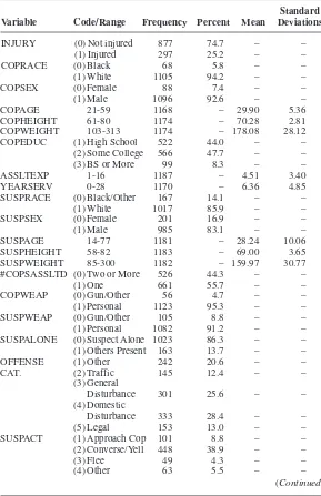
Table 1
DESCRIPTIVESTATISTICS FORMODELPREDICTINGPATROLOFFICER INJURY
Standard Variable Code/Range Frequency Percent Mean Deviations
INJURY (0) Not injured 877 74.7 – –
COPAGE 21-59 1168 – 29.90 5.36
COPHEIGHT 61-80 1174 – 70.28 2.81
COPWEIGHT 103-313 1174 – 178.08 28.12
COPEDUC (1) High School 522 44.0 – –
(2) Some College 566 47.7 – –
(3) BS or More 99 8.3 – –
ASSLTEXP 1-16 1187 – 4.51 3.40
YEARSERV 0-28 1170 – 6.36 4.85
SUSPRACE (0) Black/Other 167 14.1 – –
(1) White 1017 85.9 – –
SUSPSEX (0) Female 201 16.9 – –
(1) Male 985 83.1 – –
SUSPAGE 14-77 1181 – 28.24 10.06
SUSPHEIGHT 58-82 1183 – 69.00 3.65
SUSPWEIGHT 85-300 1182 – 159.97 30.77
#COPSASSLTD (0) Two or More 526 44.3 – –
(1) One 661 55.7 – –
COPWEAP (0) Gun/Other 56 4.7 – –
(1) Personal 1123 95.3 – –
SUSPWEAP (0) Gun/Other 105 8.8 – –
(1) Personal 1082 91.2 – –
SUSPALONE (0) Suspect Alone 1023 86.3 – – (1) Others Present 163 13.7 – –
OFFENSE (1) Other 242 20.6 – –
CAT. (2) Traffic 145 12.4 – –
(3) General
Disturbance 301 25.6 – –
(4) Domestic
Disturbance 333 28.4 – –
(5) Legal 153 13.0 – –
SUSPACT (1) Approach Cop 101 8.8 – –
(2) Converse/Yell 448 38.9 – –
(3) Flee 49 4.3 – –
(4) Other 63 5.5 – –
(1) officer and assailant attributes;
(2) situational characteristics; and
(3) environmental characteristics.
Certain officer and assailant characteristics have traditionally been thought to affect police performance. For example, it was believed Standard Variable Code/Range Frequency Percent Mean Deviations
(5) Fight/Argue 218 18.9 – –
(6) Under Arrest 272 23.6 – –
SUSPDRUNK (0) Drinking/
Intoxication 780 65.7 – –
(1) Sober 407 34.3 – –
DRUGPRES (0) No 1061 91.3 – –
(1) Yes 101 8.7 – –
PRECINCT (1) Wilkins 145 12.2 – –
(2) Woodlawn 116 9.8 – –
(3) Garrison 123 10.4 – –
(4) Towson 88 7.4 – –
(5) Cockeysville 39 3.3 – –
(6) Parkville 59 5.0 – –
(7) Fullarton 53 4.5 – –
(8) Essex 306 25.8 – –
(9)
Dundalk-Edgemere 258 21.7 – –
LOCATION (0) Outside 498 42.2 – –
(1) Inside 682 57.8 – –
SEASON (1) Winter 307 25.9 – –
(2) Spring 275 23.2 – –
(3) Summer 335 28.2 – –
(4) Fall 270 22.7 – –
DAY (1) Sunday 221 18.6 – –
(2) Monday 161 13.6 – –
(3) Tuesday 146 12.3 – –
(4) Wednesday 134 11.3 – –
(5) Thursday 146 12.3 – –
(6) Friday 170 14.3 – –
(7) Saturday 209 17.6 – –
TIME (1) 12am-8:59am 527 46.0 – –
(2) 9am-4:59pm 150 13.1 – –
that taller officers could perform certain police functions better (Bannon, 1976:70), and many line and administrative personnel still feel that female officers are unable to handle the physical aspects of police work (Charles, 1982; Grennan, 1987). Although research has generally found that individual attributes are not very important in explaining the etiology of assaults on law enforcement officers (Bannon, 1976; Uchida et al., 1989) or the use of force more generally (Croft, 1985; Friedrich, 1980), it would be premature to assume they are unrelated to the likelihood of officer injury. For example, one would expect that officers who are taller (COPHEIGHT)8and heavier (COPWEIGHT) (assuming weight is proportionate to height) have an advantage over shorter and lighter officers in protecting themselves from attack and subduing assaultive suspects.9Similarly, because males generally possess greater physical strength and are socialized more aggressively than females (Charles, 1982:19; Newman, 1979:126-36), female officers (COPSEX) may be less able than male officers to subdue assailants and more susceptible to injury when attacked.10We also expect that assailants who are taller (SUSPHEIGHT), heavier (SUSPWEIGHT) and male (SUSPSEX), will possess a greater ability to injure victim officers than their shorter, lighter and female counterparts, other things being equal.
Officer age (COPAGE) also may play a role in the probability of being injured.11Since, on average, younger officers are likely to be stronger, faster and more agile than their older counterparts, they should be better able to avoid injury when attacked. Also, we anticipate that younger assailants (SUSPAGE) will have a greater ability to injure officers than older assailants, controlling for other factors in the model.
Educational level is thought to be positively associated with police performance (Adler et al., 1994:231), but it is not clear how it might affect police assault outcomes. One correlational study, however, did find a statistically significant inverse relationship between officer education and the number of assault-related injuries (Cascio, 1977: Table 1). In view of this result, we expect to find a negative relationship between officer educational level (COPEDUC) and likelihood of injury.
Officer years of service on the force (YEARSERV) and the number of times officers reported being assaulted during the study period (ASSLTEXP) are expected to have inverse relationships with the likelihood of injury. For instance, whether through direct or indirect experience (e.g. actually being assaulted, witnessing assaults on other officers, listening to “war stories”), police may learn more effective tactics and to be more cautious when confronting assaultive suspects, thereby reducing their chances of being injured when attacked.13
Several situational variables were also selected for analysis. Wilson and Meyer (1990:43) and Grennan (1987:80-81) found that officer injury was lesslikely when encountering an armed versus an unarmed suspect, and Margarita’s (1980) research showed that high rates of injury can occur when assailants use only bodily force (Figure 5-5, p. 130). This is probably because, unlike during less overtly threatening encounters, police had some prior warning about the nature of armed situations and were more prepared (e.g. Ellis et al., 1993; Grennan, 1987). Therefore, we include the type of weapon used by the suspect (SUSPWEAP) and officer (COPWEAP),14and expect to find higher rates of officer injury when suspects use physical force to attack police. Regarding officer weapon use, a firearm or other weapon (e.g. baton, mace) should be more effective than unarmed tactics in stopping an assailant and, therefore, we anticipate armed weapon usage to be associated with a reduction in the chance of injury.15
Wilson et al. (1990:268) found that the number of officers present during an assault incident was positively associated with officer injury. While the number of nonassaulted officers present was not available in the data, we use a variable indicating whether more than one officer was assaulted at the scene (#COPSASSLTD).16Based on Wilson et al.’s (1990) results we anticipate finding a positive association between officer injury and the number of officers assaulted.17
when they confront an officer alone, thereby increasing the probability of officer injury. For instance, Toch (1980:50) writes that reasons for attacking a police officer are sometimes related to a “person’s self-image and with his appraisal of his social role”. He continues:
Even a relatively innocent inquiry by a polite officer can prompt a violent response from a person who views his manhood as challenged or his reputation as at stake. An individual contacted in public, for instance, may use the occasion to give a “benefit performance” to his potential admirers…(p. 55).
The variable DRUGPRES (whether drugs were present at the scene) was included in the model because it is conceivable that the possession of drugs may motivate assailants to attack officers more forcefully to escape and avoid a potentially more severe punishment. It is also possible that possession of drugs may be an indirect indicator of whether the suspect was under the influence of drugs, which might also affect the likelihood of officer injury (McLaughlin, 1992).18
Another variable available in the data is whether the assailant was perceived by the officer to be under the influence of alcohol (SUSPDRUNK). Alcohol use has been implicated as an instigating factor in assaults on officers (Curran et al., 1987; McLaughlin, 1992; Meyer et al., 1979; Meyer et al., 1981; Uchida and Brooks, 1988), but very few studies have examined its association with officer injury.19However, it is reasonable to assume that assaultive suspects who are intoxicated or have been drinking have less physical control and coordination than assailants who are sober, suggesting that sober assailants will be better able to injure officers.
The offense category associated with the type of offense committed by the suspect (OFFENSE CAT) was recoded into five categories (legal intervention,20domestic disturbances, other disturbances, traffic violations, and other). Because several studies have reached different conclusions regarding the dangerousness of domestic disturbances (Garner and Clemmer, 1986; Hirschel et al. 1994; Stanford and Mowry, 1990; Uchida et al., 1987), we maintained domestic and other disturbances as distinct categories. This allows us to examine the level of risk involved in the handling of domestic disputes compared to other police activities, controlling for the effects of other variables in the model.
fighting, under arrest, and other). There is little prior research to suggest how assailant actions affect the probability of officer injury, but it is arguable that situations where overt conflict is already occurring are particularly dangerous for police because it is likely they too will become a target of the suspect’s aggression (Kieselhorst, 1974:53). Therefore, we expect that suspects already involved in volatile situations (i.e. fighting/arguing) will behave more aggressively, and thus will be more likely to injure officers, than suspects engaged in less hostile actions (e.g. approaching an officer, conversing or yelling, under arrest).
Five “ecological” or environmental variables from the data set were also included in our models. First is the precinct in which the assault took place (PRECINCT). Since there was substantial variation in several socio-economic indicators across precincts in Baltimore County,21we examine whether these conditions somehow manifested themselves in the probability of officer injury. Wolfgang and Ferracuti (1982:267) relate that “within a portion of the lower class . . . there is a ‘life style,’ a culturally transmitted and shared willingness to express . . . hostile feelings in personal interaction by using physical force.” They continue, “violence . . . has been incorporated into the personality structure through childhood discipline, reinforced in juvenile peer groups, [and] confirmed in the strategies of the street.” Therefore, police assaulters from particularly violent neighborhoods may be more capable, and/or more willing, to injure officers than assailants from areas where violence is less prevalent.
We also include whether an attack took place indoors or outdoors (LOCATION). While there is no precedent to suggest how location affects the likelihood of injury during an assault, an officer’s ability to defend himself or herself may in part depend on the kind of environment in which the attack takes place. For instance, in small enclosed areas (such as a small apartment, lavatory, bar, vehicle) officers may not be able to maintain a zone of safety,22and therefore will have less time and space available for avoiding or neutralizing an attack. Confined places also may preclude the effective application of some academy-taught self-defense techniques (McLaughlin, 1992:71; Stobart, 1972:123). Therefore, we anticipate that officers assaulted indoors will be more likely to receive an injury.
association with police assaults in prior research (e.g. Bannon, 1976; McLaughlin, 1992; Meyer et al., 1981), and are therefore included here.24
Method
Because our dependent variable is binary, coded one if an officer was injured and zero otherwise, logistic regression is used to estimate the likelihood of officer injury.25The multivariate logistic regression model predicts the log-odds (the logit coefficient) of an observation being in one category of the dependent variable versus another (the reference category), given a set of explanatory variables. Continuous variables are interpreted much as in OLS regression; the logit coefficient estimates the change in the log odds of the dependent variable (i.e. officer injury) given a unit increase or decrease in an independent variable, holding constant the effects of other variables in the model. The effects of ordinal and nominal categorical variables are interpreted as the change in the log-odds of the dependent variable given a specific category of the explanatory variable.26Note, however, that a more intuitive result is obtained by exponentiating the logit coefficients to produce odds ratios. The results are then interpreted as how much the odds of an outcome change given a specific category of a categorical independent variable (or a unit increment or decrement of a continuous variable), controlling for other variables in the model (Demaris, 1992; Hosmer and Lemeshow, 1989).
On estimating our initial logistic regression models, it became apparent that the pattern of missing values exhibited in the data was problematic.27One solution was to simply proceed with the analysis using the remaining cases. However, this results in a loss of efficiency, and if the remaining cases do not comprise a random subsample of the original cases the obtained regression estimates may be biased or inconsistent (Blackhurst and Schluchter, 1989).
complete-data methods, and may give consistent results and sometimes reduce bias of parameter estimates” (Bello, 1993:855).
However, imputation methods do not perform well under all conditions (for examples, see Bello, 1993). Two such methods – mean substitution for missing data and simple replacement of missing values using regression estimates – have been shown to produce biased results and generally should be avoided (Blackhurst and Schluchter, 1989:164, 172). However, Blackhurst and Schluchter demonstrate that replacing missing values with logistic regression estimates plus a random error termperformed fairly well under a number of conditions. We therefore adopt a similar strategy for the present analysis.
It was desirable to obtain estimates for missing values for three continuous variables: officer weight (9.4% missing), officer years on the force (7.1% missing), and officer height (6.5% missing). Unfortunately, to obtain reasonable estimates of officer weight, we needed to include officer height as a predictor. Since information on officer height was missing for 77 cases, this procedure was not productive in reducing the number of missing values in the data. Therefore, prior to obtaining regression estimates of officer weight, we determined the age and sex of those officers whose values for height and weight were missing.28We then selected all officers in the complete data set that matched these cases on age and gender, calculated the mean for officer height for each group stratified by age and sex, and substituted these values for the missing data on officer height. The means, standard deviations, and other statistics for the imputed and nonimputed officer height variables were virtually identical.
Next, we regressed officer weight on officer age, height, sex and education using linear regression,29replaced the missing values for officer weight with the predicted values obtained from the regression, and then added to these values a random error term generated from a normal distribution with a mean of zero and a standard deviation equal to that obtained in the regression. The same procedure was followed for the number of years officers were on the police force (YEARSERV), which was regressed on officer age, sex, education, race, and the number of times officers were assaulted within the study period (ASSLTEXP).30
CHAID analysis to suggest how to recode the missing values. CHAID uses an imputation-like technique to merge categories of nominal or ordinal predictor variables (including missing values) that do not differ significantly from each other in terms of their relationship to the dependent variable. In other words, CHAID will merge a missing-value (or other) category with “the category with which it shares the most similar distribution of the dependent variable” (Magidson, 1993:11). The results showed that the missing values were most similar to the sober category, and the two categories were combined.31
Using the above imputed variables in a logistic regression model with all predictors reduced the number of missing cases from 371 (31.3%) to 171 (14.4%).32The findings are discussed in the following section.
RESULTS
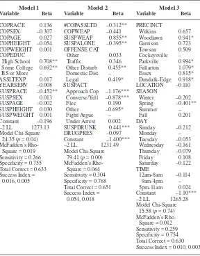
Table 2 presents the results of three logistic regressions predicting officer injury: Model 1 is comprised of officer and suspect characteristics, Model 2 consists of situational variables, and Model 3 includes environmental variables only. To conserve space at this exploratory stage, only log odds and indicators of variable significance are reported. Also note that since it is not uncommon during exploratory stages of model building to use significance levels greater than the standard 0.05 level (Hosmer and Lemeshow, 1989), we highlight those variables significant at the 0.10 level to indicate their potential importance in explaining the outcome variable. (The traditional 0.05 alpha level is used in subsequent models.) After examining each model separately, we estimate a combined model containing all independent variables (presented in Appendix A). This model is then refined (Table 3), and the implications of the findings discussed.
In examining Table 2 one sees that the situational model (Model 2) has the greatest number of predictor variables significantly related to officer injury. Specifically, Model 2 suggests that the log odds of injury increased when:
• more than one officer was assaulted (#COPASSLTD);
Table 2
ESTIMATEDCOEFFICIENTS ANDSIGNIFICANCELEVELSa FOROFFICER/ SUSPECT, SITUATIONAL ANDENVIRONMENTALMODELSPREDICTING
OFFICERINJURYb
Model 1 Model 2 Model 3
Variable Beta Variable Beta Variable Beta
COPRACE 0.136 #COPASSLTD –0.312** PRECINCT
COPSEX –0.307 COPWEAP –0.441 Wilkins 0.657
COPAGE 0.027 SUSPWEAP 0.855** Woodlawn 0.941*
COPHEIGHT –0.054 SUSPALONE –0.395** Garrison 0.723
COPWEIGHT 0.001 OFFENSE CAT Towson 0.509
COPEDUC Other 0.033 Cockeysville –
High School 0.708** Traffic 0.346 Parkville 0.994* Some College 0.692** Other Disturb 0.455** Fullarton 1.079*
BS or More – Domestic Dist – Essex 0.815*
ASSLTEXP 0.017 Legal 0.419* Dundalk-Edge 0.918*
YEARSERV –0.008 SUSPACT LOCATION –0.110
SUSPRACE –0.452** Approach Cop –1.176*** SEASON
SUSPSEX 0.013 Converse/Yell –0.878*** Winter –0.202
SUSPAGE –0.002 Flee 0.190 Spring –0.401**
SUSPHEIGHT 0.030 Other –0.695* Summer –
SUSPWEIGHT 0.001 Fight/Argue – Fall 0.201
Constant –0.196 Under Arrest 0.002 DAY
–2 LL 1273.13 SUSPDRUNK 0.441*** Sunday –0.212
Model Chi-Square DRUGPRES –0.097 Monday –
24.35 (p= 0.04) Constant –1.400*** Tuesday –0.053
McFadden’s Rho- –2 LL 1231.49 Wednesday –0.161
Square = 0.019 Model Chi-Square Thursday –0.079 Sensitivity = 0.266 79.41 (p= 0.00) Friday 0.108 Specificity = 0.755 McFadden’s Rho- Saturday –0.122 Total Correct = 0.633 Square = 0.064 TIME
Success Index = Sensitivity = 0.304 12am-8am –0.114
0.016, 0.005 Specificity = 0.768 9am-4pm –
Total Correct = 0.651 5pm-11am 0.024 Success Index = Constant –1.10***
0.054, 0.018 –2 LL 1265.28
Model Chi-Square Success Index = 0.010, 0.003
* = Significant at the 0.10 level; ** = Significant at the 0.05 level; *** = Significant at the 0.01 level
aIt is not uncommon during exploratory stages of model building to use significance levels higher than the
standard 0.05 level (Hosmer and Lemeshow, 1989). Thus, we highlight those variables significant at the 0.10 level to indicate their potentialimportance in explaining the outcome variable. The traditional 0.05 level of significance is used in the final model.
bDashed lines indicate reference categories for categorial variables; reference categories for binary
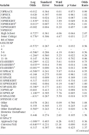
Table 3
ESTIMATEDCOEFFICIENTS, STANDARDERRORS, WALDSTATISTICS, P-VALUES, ANDODDSRATIOS FORVARIABLES IN ACOMBINEDMODEL
PREDICTINGOFFICERINJURY, INCLUDINGNONLINEARTERMSa
Log Standard Wald Odds
Variable Odds Error Statistic p-Value Ratio
COPRACE –0.012 0.364 0.01 0.973 0.99
COPSEX 0.020 0.397 0.00 0.961 1.02
COPAGE 0.042 0.024 2.94 0.087 1.04
COPHEIGHT –1.819* 0.922 3.89 0.049 0.16
COPHEIGHT2 0.013* 0.007 3.72 0.054 1.01
COPWEIGHT –0.002 0.004 0.20 0.657 1.00
COPEDUC
High School 0.727* 0.361 4.06 0.044 2.07
Some College 0.776* 0.306 4.67 0.031 2.17
BS of More – – – – –
ASSLTEXP
1-3 –0.572* 0.267 4.59 0.032 0.56
4 – – – – –
5-8 –0.586* 0.286 4.19 0.041 0.56
9-10 –1.284* 0.560 5.25 0.022 0.28
11-16 0.147 0.384 0.15 0.702 0.86
YEARSERV –0.289* 0.122 5.61 0.018 0.75
YEARSERV2 0.035** 0.014 5.98 0.014 1.04
YEARSERV3 –0.001** 0.000 6.36 0.012 0.99
SUSPRACE –0.589** 0.241 5.97 0.014 0.55
SUSPSEX –0.168 0.275 0.00 0.961 1.02
SUSPAGE 0.012 0.009 1.89 0.169 1.01
SUSPHEIGHT 0.317 0.033 0.93 0.334 1.03
SUSPWEIGHT 0.002 0.004 0.19 0.667 1.00
#COPASSLTD –0.380* 0.177 4.61 0.032 0.68
COPWEAP –0.683 0.413 2.74 0.098 0.51
SUSPWEAP 1.100** 0.395 7.76 0.005 3.01
SUSPALONE –.631* 0.267 5.59 0.018 0.53
OFFENSE CAT
Other 0.078 0.261 0.09 0.766 1.08
Traffic 0.355 0.305 1.35 0.245 1.43
Other Disturbance 0.565* 0.243 5.43 0.020 1.76
Domestic Disturbance – – – – –
Legal 0.446 0.274 2.63 0.105 1.56
SUSPACT
Approach Cop –1.008** 0.403 6.26 0.012 0.36 Converse/Yell –0.840*** 0.231 13.18 0.000 0.43
Flee 0.317 0.397 0.64 0.425 1.37
Log Standard Wald Odds
Variable Odds Error Statistic p-Value Ratio
Other –0.553 0.424 1.70 0.193 0.58
Fight/Argue – – – – –
Under Arrest 0.046 0.234 0.04 0.845 1.05
SUSPDRUNK 0.338 0.184 3.38 0.066 1.40
DRUGPRES –0.100 0.283 0.13 0.734 0.90
PRECINCT
Wilkins 1.114 0.804 1.92 0.166 3.05
Woodlawn 1.662* 0.814 4.17 0.041 5.27
Garrison 1.474 0.805 3.35 0.067 4.37
Towson 0.975 0.836 1.36 0.243 2.65
Cockeysville – – – – –
Parkville 1.807* 0.836 4.68 0.031 6.09
Fullarton 1.773* 0.845 4.40 0.036 5.89
Essex 1.588* 0.786 4.08 0.043 4.89
Dundalk-Edge 1.645* 0.788 4.36 0.037 5.18
LOCATION –0.315 0.189 2.77 0.096 0.73
SEASON
Winter –0.266 0.223 1.42 0.233 0.77
Spring –0.325 0.231 1.97 0.160 0.72
Summer – – – – –
Fall –0.211 0.231 1.22 0.270 0.78
DAY
Sunday –0.374 0.289 1.68 0.195 0.69
Monday – – – – –
Tuesday –0.358 0.321 1.24 0.265 0.70
Wednesday –0.278 0.318 0.77 0.381 0.76
Thursday –0.059 0.312 0.04 0.851 0.94
Friday 0.119 0.295 0.16 0.686 1.13
Saturday –0.179 0.288 0.38 0.535 0.84
TIME
12am-8am –0.307 0.274 1.26 0.262 0.74
9am-4pm – – – – –
5pm-11am –0.074 0.265 0.08 0.779 0.93
Constant 61.313 32.478 3.56 0.059
–2LL Constant Only Model = 1129.29 Sensitivity = 0.345 Model Chi-Square = 136.35, p= 0.000 Specificity = 0.788 McFadden’s Rho-Squared = 0.121 Total Correct = 0.680
Success Index = 0.101, 0.033
*** = Significant at the 0.05 level
*** = Significant at the 0.01 level *** = Significant at the 0.001 level
aDashed lines indicate reference categories for categorical variables; reference categories for binary
• the assailant was not accompanied by other suspects (SUSPALONE);
• officers responded to other disturbances and legal situations versus domestic disturbances (OFFENSE CAT);
• suspects were under arrest, attempting to escape, or were fighting/arguing compared to when they were conversing/yelling, approaching an officer, or involved in some “other” action (SUSPACT); and
• officers reported assailants as being sober. (We postpone an interpretation of the results until after the final model is estimated.)
Model 1 (officer/suspect attributes) produced only two predictors significantly related to the dependent variable. Here we find an increase in the log odds of injury when officers had less than a four-year college degree (COPEDUC), and when assailants were nonwhite (SUSPRACE).
Model 3 suggests that, compared to Cockeysville, the risk of injury is significantly greater for patrol officers assaulted in five of the other precincts (PRECINCT), and when officers were assaulted in the summer versus the spring months (SEASON). Note, however, the model chi-square value indicates that none of the coefficients in this model are significantly different from zero.33 McFadden’s Rho-squared and the other statistics34reported at the bottom of each model also indicate that the environmental model performs the worst while the situational model performs best in explaining officer injury.
We also wanted to examine more closely the effect of ASSLTEXP, the number of times officers were assaulted within the three-year study period. If one suspects that a continuous explanatory variable is related to the criterion nonlinearly, one option is to group the variable into categories and proceed with the analysis (Hosmer and Lemeshow, 1989:57; Pedhazur, 1982:404). Therefore, because ASSLTEXP was fairly limited in range36we decided it should be recoded and treated as a categorical variable (as opposed to attempting to model it nonlinearly with power polynomials or transformations).37Given that we found statistically significant nonlinear effects, we limit our discussion to the results displayed in Table 3 (for those interested, however, the combined linear model appears in Appendix A).
As shown in Table 3, the variables that were statistically significant in the individual attributes model (Model 1, Table 2) remain significant and relatively unchanged in magnitude. In addition, however, significant nonlinear effects were obtained for officer height (COPHEIGHT) and years of service (YEARSERV). For COPHEIGHT we find that for each inch increase in officer height there is a large and statistically significant decrease in the odds of officer injury. However, while taller officers have a lower associated risk of injury, the statistically significant second-order term indicates that height has a diminishing impact on the odds of injury with greater increases in officer height. For each additional year of service (YEARSERV) the odds of an officer receiving an assault-related injury also decrease significantly and substantially. Examination of the quadratic and cubic terms, however, suggest that the odds of injury increase, and then decline again with additional years of service. (We clarify the nature of these nonlinear relationships in the discussion section.)
(SUSPAGE), officer weight (COPWEIGHT), suspect weight (SUSPWEIGHT), and suspect height (SUSPHEIGHT).
Among the environmental factors in the combined model, the time, day, season and location of the assault were unrelated to officer injury. Note that the statistically significant difference between the spring and summer categories for SEASON in Model 3 (Table 2) became non-significant once additional variables were controlled for. The effect of neighborhood or community context (PRECINCT), however, appears to be important in terms of risk of injury, with the estimates increasing substantially in magnitude and statistical significance in the combined model. One sees that, compared to officers assaulted in Cockeysville, the odds of injury were much greater among officers assaulted in five other precincts.
A comparison of the values for McFadden’s Rho-squared and the Success Index obtained in the combined model in Table 3 indicates substantial improvement over each of the three individual models shown in Table 2. However, the magnitude of McFadden’s Rho-squared for the combined model (0.12) suggests only a modest result. The prediction success table results also are not terribly optimistic; the combined model correctly predicted only 86 (35%) of the observed 248 injured officers.39 Moreover, the combined model showed only a moderate increase over the individual models in the proportion injured correctly predicted (about a 10 percent increase over Models 1 and 3, but only a five percent increase over Model 2). Nevertheless, the results do suggest which variables are important in their own right in explaining officer injury.
DISCUSSION
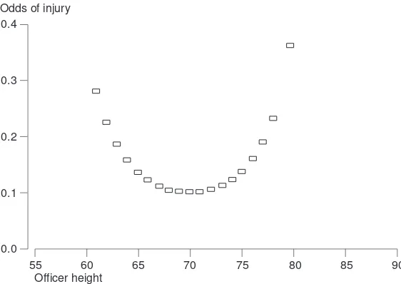
However, contrary to our expectations, most officer and suspect characteristics were unrelated to officer injury in our analysis. For example, we found (as did Grennan, 1987:80-81) that female officers were no more likely to be injured when assaulted than male officers, indicating that line and administrative concerns about female officers being unable to handle violent encounters maybe unjustified.40The sex of the assailant was not a factor in causing officer injury either, implying that assaultive women should be considered no less dangerous than assaultive men.
Other physical characteristics commonly believed to be associated with injury were insignificant as well. For example, the weight41and age of officers and assailants were statistically unrelated to officer injury. However, officer height (but not assailant height) was significant. Figure 1 depicts this relationship by plotting officer height against the predicted odds of injury, calculated for each value of height in the data. One sees that the odds of injury decrease as officer height increases, but only up to 70 inches; the odds of injury then begin to increase for officers taller than 70 inches. Thus, officers who are 70
0.4
0.3
0.2
0.1
0.0
Odds of injury
55 60 65 70 75 80 85 90
Officer height
Log odds of injury = 61.313 – 1.819 (officer height) + 0.013 (officer height)2
Figure 1:
inches tall have the lowest possible risk of injury, while the tallest officers (80 inches) have the highest risk.42It is unclear whether this finding is due to the characteristics of the officers (e.g. shorter officers being less able to defend themselves) and/or to the motivations and strategies of assailants (e.g. launching particularly forceful attacks on very tall officers to ensure victory), or both.
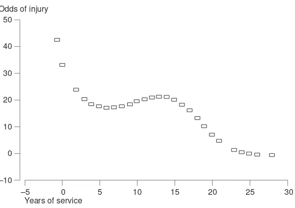
The odds of injury decreased as officers gained more experience on the job, but as with officer height the relationship is complex. Figure 2 shows that the odds of injury decline rather sharply as officers gain experience during their first six years on the job. However, further reductions in the odds of injury occur only at much greater levels of experience – starting at about the 13th year.43
Officer race was unrelated to injury, but patrol officers were more likely to be injured when assaulted by nonwhite suspects than when attacked by white suspects. It is difficult to develop an adequate explanation for this finding without additional information. However,
50
40
30
20
10
0
–10
Odds of injury
–5 0 5 10 15 20 25 30
Years of service
Log odds of injury = 61.313 – 0.289 (years of service) + 0.035 (years of service)2 – 0.001(years of service)3
Note: Odds in this graph have been divided by 1E+25 to facilitate plotting Figure 2:
because of the historically antagonistic relationship between the police and minority communities (Hochstedler and Conley, 1986; Murty et al., 1990), many minorities hold less favorable attitudes toward the police than do whites (Bouma, 1973; Decker, 1985; Smith et al., 1991). Therefore, attacks on police by nonwhite assailants may tend to be particularly contentious.44
Officers with four or more years of college education were less likely to be injured when attacked than officers with less than four years of college experience or only a high school education, results congruent with Cascio’s (1977) finding of an inverse relationship between officer injury and officer education in Dade County, Florida. Although speculation, education may somehow be positively associated with cautionary behaviors on the part of officers, thereby reducing their chances of being injured when assaulted.
We also expected to find a reduction in the odds of injury with increases in the number of times officers were assaulted within the study period. Here we assumed that officers would be better prepared to handle such attacks as their experience with them increased. We did find that compared to officers assaulted four times, those assaulted five to eight times and nine to ten times were significantly less likely to be injured, providing partial support for our hypothesis. However, we also found that officers assaulted one to three times were less likelyto be injured than officers assaulted four times, a relationship counter to our hypothesis.45
Several situational characteristics were associated with the likelihood of officer injury, and based on the model statistics (Models 1-3 in Table 2) they performed best overall in explaining injury. We found that injury was positively associated with multiple-victim assault incidents, indicating that single-victim officers were less likely to be injured. Perhaps unaccompanied officers interviewing and confronting suspects take more precautions than when other officers are present, or maybe assailants brazen enough to attack multiple police officers represent particularly dangerous threats. This variable does, however, suffer from measurement problems and should be viewed cautiously.47
Officers were more likely to be injured when assailants used bodily force as opposed to a firearm or other weapon. There may be a couple of reasons for this. First, although gunshot wounds pose a serious threat to police, only two (5.4%) out of 37 gun assault victims were injured, and of these only one was hospitalized. However, none of the officers shot at were hit (Uchida and Brooks, 1988:31). The high failure rate of the gun assaults (and to a lesser degree other weapon assaults)48 suggests that officers had prior warning that they might be facing armed situations and took appropriate defensive measures.
Second, the high injury rate from unarmed attacks may reflect partially the less predictable nature of such events. For example, McMurray (1990:57) found that 74 percent of a sample of assaulted officers in Washington, DC, and Newark, NJ, were disturbed most about the unpredictable nature of their assaults, suggesting that the officers had not anticipated being attacked. Meyer (1992:10) characterizes many police use-of-force situations as “sudden, close-contact situations requiring immediate, instinctive response,” indicating there is often little warning that an attack is imminent. We also suspect that there is an “habituation effect,” i.e. where officers so frequently encounter situations in which the potential for use of force exists, but where force (beyond a firm grip) is not used that they come to expect most routine situations will be resolved without physical conflict, and therefore become less cautious over time. Thus, taking greater precautions during more routine encounters may do much to reduce the number of successful assaults.
explanation requires more specific information about the actions (if any) taken by other suspects or anyone else present at the scene (e.g. bystanders, family members).
Ellis et al. (1993), Stanford and Mowry (1990), and Uchida et al. (1987) found that domestic disturbances were more injurious than other disturbances; however, we found just the opposite. Furthermore, our research showed that domestic disturbance assaults were no more injurious than assaults occurring during legal interventions or when officers responded to traffic violations. Although the Stanford and Mowry (1990) and Uchida et al. (1987) studies are noteworthy, their estimates of danger rates for various police activities fail to control for the effects of other variables that may be important in explaining the likelihood of officer injury. Similarly, although Ellis et al. (1993) used multivariate techniques, they examined the effects of officer attributes and situational characteristics on injury in separate models, and did not include offender characteristics or environmental factors.49Thus, our risk estimates may be the most accurate to date.
The actions taken by suspects prior to assaulting officers also seem to be important in explaining the likelihood of officer injury. For instance, officers were less likely to be injured when approached by suspects, and when suspects were conversing/yelling as compared to when they were already fighting with or arguing with another officer. Other actions, such as when offenders were trying to escape or were under arrest, were about as dangerous to officers as when offenders were fighting. Thus, apprehended offenders, escape attempts, and police-citizen conflicts appear to represent more volatile, fight-or-flight situations, suggesting that law enforcement officers should be particularly cautious when dealing with suspects in these circumstances. The estimate of the effect of suspect alcohol use on injury, although technically only near statistical significance, nevertheless supports our notion that assailants under the influence of alcohol are less able than sober assailants to carry out successful assaults (see note 42). However, since only one other study has examined the relationship between suspect alcohol use and officer injury and found no effect (Ellis et al., 1993), further study on the role alcohol plays in assault outcomes is needed.
proxy variable – whether drugs were present at the scene of the assault – proved to be statistically unrelated to the outcome variable.
The sign of the coefficient for the remaining situational variable – the type of weapon used by the officer (bodily force or other weapon) – was negative and in a direction opposite of that anticipated. Though insignificant (p= 0.098), the direction of the effect suggests that officers were less likely to be injured when they used physical force compared to when they used a firearm or other weapon. It is important that future research examine the relationship between type of officer weapon use and the probability of injury to determine which weapons provide the most safety for police, especially as new nonlethal weapons (e.g. oleoresin capsicum sprays, side-handle batons) are developed and issued to police on a wider basis.
Policy Implications
The results of this study suggest several implications for policy.50 First, the data show that the majority of assault incidents involved unarmed attacks against the police, and that such attacks were more likely to result in officer injury than armed attacks. Moreover, most officers responded to assailants with physical force. Batons, firearms, or other weapons were rarely used. Thus, greater officer proficiency51in unarmed defensive tactics may help reduce the number of police assault-related injuries.
Second, since fewer years of service was associated with increases in risk of injury, police departments might consider providing additional in-service training for patrol officers with less than five or six years of experience to ensure adequate skill acquisition and retention in use-of-force prevention strategies and unarmed defensive tactics. In-service training for more experienced patrol officers might still be desirable, but could be conducted less frequently. The reductions in work time lost and medical costs due to injuries may well offset the costs of instituting such a program.
strategies to increase these officers’ effectiveness during use-of-force encounters.
Fourth, substantial numbers of assaulted officers reported being victims multiple times within the study period. Therefore, it may be beneficial for police administrators to identify such officers, as well as those repeatedly involved in use-of-force conflicts more generally. Departments could then work with them to reduce their involvement in use-of-force encounters. Toch and Grant (1982) implemented this type of program in the Oakland Police Department in California.
Fifth, the actions taken by assailants prior to assaulting officers indicate that the risk of injury is, to some degree, associated with suspect motivation. Specifically, the data suggest that suspects already involved in hostile conflicts with other officers, escape attempts, and arrest situations represent increased risks to police, calling for greater caution from officers facing these kinds of situations.
Sixth, officers assaulted by nonwhite suspects were more likely to be injured than officers assaulted by white suspects, suggesting that these incidents were characterized by greater hostility. Although instruction in violence-reduction strategies in general is important for recruits and patrol officers, additional attention should be paid to police and minority community relations and awareness programs to reduce tensions and hostilities.
Seventh, officers graduating college were less likely to be injured than officers without a degree. Lower injury rates among better educated officers, possibly due to greater caution and/or foresight, suggest one more reason for law enforcement to continue the trend toward higher education.
NOTES
An earlier version of this paper was presented at the annual meeting of the American Society of Criminology, Miami, November 9-12, 1994. The data utilized in this analysis, originally collected by Craig D. Uchida and Laure W. Brooks, were obtained from the Inter-university Consortium for Political and Social Research. We thank David McDowall and the anonymous reviewers for their helpful comments. Of course, we bear full responsibility for the analyses, interpretations and any errors presented herein.
1. For instance, Stobart (1972:111) reported 10,935 work days lost in one year alone due to injurious assaults on officers in one large municipal agency.
2. At the time of Bard’s analysis, the UCR defined “disturbance calls” as “family quarrels, man with gun, etc.” While the disturbance call category in fact represented an aggregation of different types of disturbances, it was often perceived by laymen and researchers alike as referring solely or mostly to domestic disturbances. This aggregation and associated misconception inflated the apparent “dangerousness” of the domestic disturbance call (Garner and Clemmer, 1986:2).
3. Other calls for service examined by Hirschel et al. (1994) were burglaries, robberies, other arrests, suspicious persons/ circumstances, mentally deranged, handling prisoners, traffic stops, and other (p. 109).
relevant variables from their model, such as officer and assailant characteristics. Omitting relevant variables also can result in model misspecification (Pedhazur, 1982:225-230).
5. Ninety-three percent of the BCPD law enforcement officers assaulted were patrol officers.
6. Ninety-seven percent of the BCPD officers were in uniform, and 98.6 percent were on patrol duty at the time they were assaulted.
7. After making the other selections, only 4.1 percent (54) of the assaults involved more than one assailant.
8. Note, though, that after an extensive review of the literature and an examination of data from five law enforcement agencies, White and Bloch (1975:6) concluded that there were no “important difference[s] in the performance of tall and short officers with similar seniority and assignments,” including the likelihood of officer injury. However, the statistical methods used were rather simple – specifically, the Kolmogorov-Smirnov Two-Sample Test and chi-square tests of significance (p. 93) – and the data were often so inadequate that no firm conclusions could be reached (pp. 6,14).
9. Of course, physical size and strength are not likely to be important determinants of officer and assailant accuracy with a firearm. Thus, this and related arguments assume that assailants typically use “personal” weapons to attack officers (i.e. fists, feet, or other bodily force), and that officers typically respond to these attacks with personal weapons themselves. This is certainly true in this study (91.2 percent of the suspects and 95.3 percent of the officers used only physical force), and nationally as well (for example, see Flanagan and MaGuire, 1992:420; Meyer et al., 1979; McEwen and Leahy, 1993:2; Pate and Fridell, 1993b:9).
11. The effect of officer age may become more salient if police departments eliminate current age requirements for applicants, as the LAPD did recently.
12. All of the nonwhite officers in the analysis were African-American, and all but three of the nonwhite assailants were African-American.
13. It is also important to include this variable in the model because it controls for the fact that the observations may not be fully independent, i.e. that there are multiple victimizations of some officers.
14. It was necessary to combine the firearm and other weapon categories as there were too few cases for analysis after taking into consideration missing values; for officers, 3.6 percent (42) used a firearm, and 1.2 percent (14) some other weapon; for suspects, 3.1 percent (37) used a firearm and 5.7 percent (68) some other weapon.
15. This, of course, assumes that officers did not draw their weapon subsequent to being attacked and injured.
16. Note that officers were assigned to single-unit patrols at the time of the study.
17. It is probable that the same process is at work for both the number of assaulted and unassaulted officers present at the scene, i.e. that other officers respond to or are dispatched to more volatile situations.
18. The direction of the effect of a specific drug is difficult to determine, however, as it can vary depending on the physical, mental and emotional characteristics of an individual. Certain drugs, though, have been known to increase physical strength and insensitivity to pain, e.g. anabolic steroids and PCP (McLaughlin, 1992:79-80).
actually be under the influence of alcohol at the time of the assault. As the authors note, this variable represents assailants who “have a drinking problem and/or have been drinking” (p.159).
20. Legal intervention refers to “executing search and arrest warrants, transporting prisoners, conducting jail searches, and backing up officers” (Uchida and Brooks, 1988:28).
21. Uchida et al. (1989) used census data to describe the socio-economic context of each of the nine precincts in Baltimore County. Essex and Dundalk-Edgemere had the highest violent crime rate, lowest median income, lowest average years of education, highest percent unemployment, highest number of assaults per officer, and a 93 percent white population. Cockeysville had the most positive average ranking based on the socio-economic indicators, and had a population that was 96 percent white. Woodlawn and Garrison had the largest African-American populations (28 percent and 13 percent, respectively), and had moderate rankings based on the socio-economic indicators. Fullarton and Parkville were 95 percent white and generally had high rankings, although not as high as Cockeysville (Table 2).
22. When interviewing suspects, law enforcement officers often are taught to maintain a certain distance between themselves and the persons they are interviewing. This gives the officer more time to react to an assault, and increases his or her chances of evading or countering a suspect’s kick, punch, or other offensive movement (Clede and Parsons, 1987:31).
23. However, lighting and weather conditions could conceivably have some effect on use-of-force outcomes.
24. Although the inclusion of variables with no theoretical expectations in a regression model (sometimes referred to as “kitchen sink models”) may be objectionable, the inclusion of irrelevant variables does not lead to bias in the estimates of regression coefficients (Pedhazur, 1982:228-229).
assumptions. Although discriminant analysis might be used, it assumes multivariate normality of the independent variables (Demaris, 1992), which may not be reasonable, especially when qualitative explanatory variables are included in a model (Kennedy, 1992:236).
26. For categorical variables in this analysis we use an indicator-variable coding scheme, which estimates the effect of a particular category of an explanatory variable on the dependent variable compared to a specific reference category. One alternative is to compare the effect of each category of an independent variable to the average effect of all the categories of that variable (see Norusis, 1993 for an example).
27. In a model containing all the variables, 371 cases (31.3%) were eliminated listwise due to missing data.
28. We selected cases where officer height andweight were missing (n= 64) to keep at a minimum the number of cases for which we would have to estimate values for height; thus, we estimated height values for 64 officers instead of all 77.
29. All predictors were significant at or less than p= 0.0001; the R Squared value was 0.46.
30. All predictors were significant at or less than p= 0.0002; the R Squared value was 0.61.
31. It is possible that officers assaulted by suspects who were perceived not to be under the influence of alcohol were more likely to omit that information from their reports than in those situations where suspects were believed to be under the influence of alcohol. This may explain why the distributions of the missing and sober categories were similar in relation to the dependent variable.
33. The interpretation of the model chi-square value in logistic regression is analogous to the overall Ftest in linear regression, and if significant indicates that one or more coefficients in the model are different from zero (Hosmer and Lemeshow, 1989:31).
34. McFadden’s Rho-squared mimics R-squared but tends to be much lower in magnitude; values between 0.20 and 0.40 are considered to be very good. Sensitivity and specificity are based on a prediction success table: Sensitivity is the proportion of the injured officers correctly predicted (i.e. response cases); Specificity is the proportion of those officers not injured correctly predicted (i.e. reference cases); the Total Correct figure is the total cases successfully predicted; the Success Index is a measure of the gain achieved by the model for responses and references, respectively, over a model with only a constant. Smaller values indicate poorer model performance (Steinberg and Colla, 1991).
35. Briefly, one recodes a continuous variable into quartiles or quintiles, replaces the original variable with the categorized variable in the logistic regression, and then plots the logits obtained from the regression against the medians of the groupings. The resulting pattern then suggests the nature of the relationship between the independent variable of interest and the dependent variable.
36. ASSLTEXP originally had 15 categories with a range of 1 to 16 assaults.
37. ASSLTEXP was recoded into five categories, which were arrived at by successively treating each category as the reference and merging adjacent categories that were not significantly different from it, but keeping separate those categories that were found to be statistically significant from at least one other category (e.g. this is why category 2 – those assaulted four times – was not merged with category 1 – those assaulted one to three times).
39. There were 248 injured officers in the logistic regression analysis after deletion of cases with missing values.
40. However, we feel that before firm conclusions regarding female officer safety can be made, a closer examination of the dynamics of assault incidents is warranted. For instance, male officers may tend to take command of potentially violent situations (Grennan, 1987:79), thereby reducing the risk of injury to female officers. Additionally, the majority of injuries in this study were minor, and significant gender differences might be found if injury seriousness was the focus of a study.
41. We also computed bodymass variables that took into account the weight andheight of officers and suspects, but they failed to achieve statistical significance.
42. Computing odds ratios, we find that the odds of injury for an officer 80 inches tall are about 3.7 times those for an officer 70 inches tall, while the odds of injury for an officer 61 inches tall are about 2.8 times those for an officer 70 inches tall. Although the tallest officers have the highest risk of injury, the odds of injury for an officer 81 inches tall are only 1.30 times those for an officer 61 inches tall.
43. Calculating odds ratios, we find that an officer with less than one year of service is 13.5 times as likely to be injured as an officer with 28 years of service; an officer with six years of service is 6.8 times as likely to be injured as is an officer with 28 years of service.
44. One of the anonymous reviewers also suggested a “victim precipitation” explanation, i.e. that officers using greater force against nonwhite suspects may be increasing their own risk of injury. On the other hand, one could argue that officer use of greater force during physical encounters mightreducetheir risk of injury.
disadvantage they incur in not having alleged an attack upon themselves in which they were required to use force in order to overcome . . . resistance”. Therefore, some number of alleged assaults probably did not occur. Although both problems threaten the validity and reliability of the data, the truncation problem is probably the more serious of the two.
46. A potential problem in relating police injury rates to socio-demographic characteristics of precincts in regression is that the residuals may be spatially autocorrelated. Precinct boundaries are artificially created, likely causing some socially, demographically, and culturally homogenous neighborhoods to be intersected by these boundaries. Therefore, socio-demographic measures in one precinct are unlikely to be independent of the same measures in adjacent precincts resulting in spatial autocorrelation. This can cause the standard errors of the regression coefficients to be biased, thus affecting the tests of significance of the regression estimates (Odland, 1988).
47. We are unable to tell from the data if in fact single-victim assault incidents are less dangerous than incidents where multiple officers are assaulted. To answer this question appropriately requires information about:
• whether other officers were present at the initiationof an assault incident and immediately assisted a victim-officer;
• whether other officers assisted a victim-officer subsequent to the initiation of the assault; and
• the number of assisting officers assaulted and their injury status.
48. Of 68 attacks where assailants used some other weapon, only 13 (19.0%) of the officers were injured, and of these five were hospitalized; of the 1,070 officers attacked by unarmed suspects, 282 (26.4 %) were injured and 43 hospitalized.
49. The exclusion of variables related to both the criterion and other explanatory factors in a model leads to model misspecification and biased parameter estimates (Pedhazur, 1982:226).
probability of being assaulted in the first place. For instance, we found that very tall officers were more likely to be injured when assaulted than officers of average height. However, if taller officers are much less likely to be assaulted in the first place, their overalllikelihood of injury would be low. Thus, the inferences one can make from the given data are more limited than if the sample were comprised of assaulted and unassaulted officers.
51. It appears that most police recruits receive relatively few hours of unarmed defensive tactics training. For example, the minimum number of hours of instruction mandated by New York State, Massachusetts, Michigan, and Washington range from 35 to 48 hours, with no in-service training required (Bruining, 1994; Hodges, 1994; Large, 1994; Wayne, 1994). Most large city and county police departments (i.e. those with 500 or more sworn personnel) conduct their own training, with some providing more hours of instruction than mandated by the state. For instance, the SFPD provides their recruits with 148 hours of instruction, and the Honolulu PD provides about 100 hours. However, on average, most large agencies provide about 62 hours of unarmed defensive tactics training; the Washington, DC Metropolitan Police Department provides only 10 hours (Strawbridge and Strawbridge, 1990). Thus, even among large agencies it is doubtful that many patrol officers will develop and retain appropriate skill levels without more hours of academy instruction and regular in-service training (McLaughlin, 1992:119).
REFERENCES AND FURTHER READING
Adler, F., Mueller, G.O. and Laufer, W.S. (1994), Criminal Justice, New York, NY: McGraw-Hill, Inc.
Aldrich, J.H. and Nelson, F.D. (1984), Linear Probability, Logit, and Probit Models, Beverly Hills, CA: Sage Publications.
Bard, M. (1970), Training Police as Specialists in Family Crisis Intervention, Washington, DC: U.S. Government Printing Office.
Bello, A.L. (1993), “Choosing Among Imputation Techniques for Incomplete Multivariate Data: A Simulation Study”, Communication in Statistics – Theory, 22(3): 853-877.
Bouma, D.H. (1973), “Youth Attitudes Toward the Police and Law Enforcement”, in Curran, J.T. et al. (Ed), Police and Law Enforcement: 1972, New York, NY, AMS Press, Inc.
Blackhurst, D.W. and Schluchter, M.D. (1989), “Logistic Regression with a Partially Observed Covariate”, Communication in Statistics – Simulation, 18(1): 163-177.
Boylen, M. and Little, R.E. (1990), “How Criminal Justice Theory Can Aid Our Understanding of Assault on Police Officers”, The Police Journal, 63(3): 208-215.
Bruining, H. (1994), Telephone interview, January 18, Michigan Law Enforcement Training Council and State Police Academy, MI.
Cascio, W.F. (1977), “Formal Education and Police Officer Performance”,
Journal of Police Science and Administration, 5(1): 89-96.
Charles, M.T. (1982), “Women in Policing: The Physical Aspect”, Journal of Police Science and Administration, 10(2): 194-205.
Clede, B. and Parsons, K. (1987), Police Nonlethal Force Manual: Your Choices This Side of Deadly, Harrisburg, PA: Stackpole Books.
Croft, E.B. (1985), “Police Use of Force: An Empirical Analysis”, Ph.D. dissertation, State University of New York at Albany, Ann Arbor, MI; University Microfilms International.
Curran, P.J., Dodds, R., Edwards, F., Hastings, T. and Schwartz, R. (1987), Report to the Governor: New York State Commission on Criminal Justice and the Use of Force, Volumes I and III, May.
Decker, S.H. (1985), “The Police and the Public: Perceptions and Policy Recommendations”, in Homant, R.J. and Kennedy, D.B. (Eds), Police and Law Enforcement: 1975-1981, Vol. 3, New York, NY: AMS Press, Inc.