Parameter estimation of two-fluid capillary
pressure–saturation and permeability functions
J. Chen, J.W. Hopmans* & M.E. Grismer
University of California, Department of Land, Air & Water Resources, Hydrology Program, 123 Veihmeyer, Davis, CA 95616, USA
(Received 17 December 1997; revised 17 June 1998; accepted 27 June 1998)
Accurate characterization and modeling of subsurface flow in multi-fluid soil systems require development of a rapid, reproducible experimental method that yields the information necessary to determine the parameters of the capillary pressure–saturation and permeability functions. Previous work has demonstrated that parameter optimization using inverse modeling is a powerful approach to indirectly determine these constitutive relationships for air–water systems. We consider extension of the inverse parameter estimation method to the modified multi-step outflow method for two-fluid (air–water, air–oil and oil–water) flow systems. The wellposedness of the proposed parameter estimation problem is evaluated by its accuracy, uniqueness and parameter uncertainty. Seven different parametric models for the capillary pressure– saturation and permeability functions were tested in their ability to fit the multi-step outflow experimental data; these included the van Genuchten–Mualem (VGM) model, van Genuchten–Burdine (VGB), Brooks–Corey–Mualem (BCM), Brooks–Corey– Burdine (BCB), Brutsaert–Burdine (BRB), Gardner–Mualem (GDM) and Lognormal Distribution–Mualem (LNM) models. The VGB, BCM and BCB models fitted the multi-step outflow data poorly, and resulted in relatively large values for the root-mean-squared residuals. It was concluded that the remaining VGM, LNM, BRB and GDM models successfully characterized the multi-step experimental data for two-fluid flow systems. Although having one parameter less than the other models, the GDM model’s performance was excellent. Finally, we conclude that optimized capillary pressure–saturation functions for the oil–water and air–oil could be predicted from the respective air–water function using interfacial tension ratios. q1999 Elsevier Science Ltd. All rights reserved.
1 INTRODUCTION
Successful environmental protection and remediation stra-tegies associated with hydrocarbon contamination of soil and ground water requires modeling of multi-fluid flow and transport in subsurface soil systems. However, the implementation of such models is often hampered by lack of sufficient information regarding the capillary pressure– saturation and permeability functions for the different soil materials.
Methods to determine soil capillary pressure and perme-ability functions are either based on measurements or are partially derived from prediction models. Equilibrium and steady-state experimental methods are usually highly restrictive by constrained initial and boundary conditions,
time-consuming, and can often not be replicated1–3. Predic-tion methods4,5are typically based on a simplified concep-tual soil pore model for predicting permeability from pore-size distribution information obtained from capillary pres-sure–saturation data. Alternatively, the similarity assump-tion is applied to predict unknown capillary pressure or permeability functions from known values of easy-to-mea-sure soil or fluid properties6,7. In either case, independent data are required to test the validity of the prediction models.
In recent years, the parameter estimation approach in combination with inverse flow modeling has been devel-oped to complement existing measurement and predictive methods for estimation of the constitutive relationships for air–water systems. Advantages of the parameter estimation method include: (1) the experiment for which the modeling is to be conducted may be transient, and thereby faster than q1999 Elsevier Science Ltd Printed in Great Britain. All rights reserved 0309-1708/99/$ - see front matter
PII: S 0 3 0 9 - 1 7 0 8 ( 9 8 ) 0 0 0 2 5 - 6
steady-state methods; (2) boundary and initial conditions of the experiment can be freely chosen; and (3) both the capillary pressure–saturation and permeability function parameters are obtained simultaneously for the same soil sample. Estimation of the constitutive functions for air–water systems using the inverse method has become increasingly attractive8–17. The fundamental assumption of inverse modeling parameter estimation is that the consti-tutive functions can be described by a parametric model for which the unknown parameters can be estimated by mini-mization of deviations between observed and predicted state variables such as flux density or capillary pressure. To deter-mine whether the inverse problem can be solved, it must be ‘correctly posed’18. Ill-posed inverse problems may result in no solution, non-uniqueness (more than one solution), or instability (solution is sensitive to small changes in input data).
Previous studies have shown that the experimental method plays an important role in determining the well-posedness of the parameter estimation problem and indicated that a minimum amount of data must be collected to characterize the simulated flow process. For example, Gardner’s19 one-step transient outflow method may be an ill-posed parameter estimation problem, yielding a non-unique set of parameters for the constitutive relationships. Van Dam et al.20 suggested that cumulative outflow be measured during multiple outflow steps, so as to yield suffi-cient information for determination of a unique parameter set using the inverse method. Including capillary pressure measurements during the outflow experiment further resulted in improved parameter sensitivity15. Also, Eching and Hopmans9 concluded that measurement of capillary pressure in addition to outflow measurements provided
adequate information for unique solutions of the inverse parameter estimation problem.
Although inverse parameter estimation approaches have been developed and increasingly applied in recent years, their application has been limited to air–water flow soil systems. In the modeling of these soil systems, the tradi-tional Richards’ assumption of neglecting the influence of the air phase on water flow is applied. Here, we expand application of the inverse parameter estimation method to other two-fluid flow systems, including air–oil and oil– water. We examine use of the inverse parameter estimation method, using two-fluid multi-step outflow experiments in conjunction with numerical solution of the two-fluid flow equations, to determine the parameters characterizing the constitutive relationships for multi-fluid flow systems. We first use the van Genuchten–Mualem functions because of their proven fitting ability and widespread use, and their successful application by Eching et al.10 to the results of multi-step outflow experiments for air–water systems. We also evaluate the application of the van Genuchten–Burdine (VGB), Brooks–Corey–Mualem (BCM), Brooks–Corey– Burdine (BCB), Brutsaert–Burdine (BRB), Gardner– Mualem (GDM) and lognormal distribution–Mualem (LNM) relationships in the inverse method.
Russo and associates21,14studied the applicability of var-ious constitutive hydraulic relationships for air–water sys-tems, whereas Demond and Roberts2 compared various parametric models for general two-fluid flow systems. How-ever, to date no information is available on the applicability of different constitutive relationships for parameter estima-tion of multi-fluid flow systems. Consequently, in addiestima-tion to evaluating the use of the multi-step outflow method in conjunction with the inverse parameter estimation technique
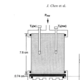
Fig. 1. Experimental setup for multi-step outflow. Pressure transducers T2and T3measured the wetting (w) and non-wetting (nw) fluid
for estimating constitutive relationship parameters of multi-fluid flow systems, we also consider the applicability of several different capillary pressure–saturation and perme-ability relationships to this approach.
2 MATERIALS AND METHODS
2.1 Experimental apparatus
Multi-step transient outflow experiments were modified from Eching and Hopmans9,10to include measurement of the non-wetting fluid pressure (Fig. 1), and were conducted in a constant-temperature (208C) laboratory22. Soils used in
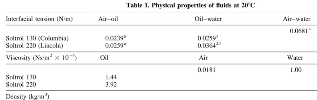
the transient outflow experiments were air-dried, sieved to less than 2 mm in diameter, and uniformly packed in a 6.0 cm inside-diameter and 7.6 cm high brass soil core that was placed in a standard Tempe pressure cell. Two soils, a Columbia fine sandy loam (63.2% sand, 27.5% silt and 9.3% clay) and a Lincoln sand (88.6% sand, 9.4% silt and 2.0% clay) were used in the multi-step experiments. These experiments were conducted using air or oil as the non-wetting (nw) fluid, displacing either water, or oil as the wetting (w) fluid, assuming one-dimensional vertical flow in the soil core. Soltrol 130 and Soltrol 220 were used as the oil phase for the Columbia and Lincoln soils, respectively. The density, viscosity, and interfacial tension values for the experimental fluids are listed in Table 1. A 0.74 cm thick porous ceramic plate at the base of the soil core allowed drainage of the wetting fluid, but was impermeable to the non-wetting fluid.
Applied air pressures (expressed in cm water height) for the air–water system were 60, 80, 120, 200, 400, and 700 cm above atmospheric pressure for the Columbia soil. Selected equivalent air pressure steps for air–water of the Lincoln soil were 40, 60, 80, 100, 150, 200 and 400 cm above atmospheric pressure. These steps were smaller than those for Columbia soil, because of Lincoln soil’s coarser texture. For both soil types, applied air pressure
increments were chosen such that drainage volumes were approximately equal for each pressure step. The pressure steps for the other fluid pairs were reduced, to account for differences in interfacial tension values between the tested fluid pair and air–water, thereby creating approximately equal drainage volumes for each wetting fluid during each pressure step. A pressure step increment required from 5 to 36 h to reach equilibrium or near-equilibrium conditions, depending on the pressure of the wetting fluid and soil type. After the drainage rate reduced to near zero, the non-wetting fluid pressure was incrementally increased for the next drainage step. Initially the soil was fully saturated with the wetting fluid, and then subsequently drained to a saturation corresponding to slightly in excess of the non-wetting fluid entry pressure, thereby ensuring continuity of the non-wetting fluid throughout the soil core at the onset of wetting fluid displacement24. Both cumulative outflow from the base of the soil core and pressures of both the wetting and non-wetting fluid at the center of soil core were measured continuously using pressure transducers (T1, T2and T3in Fig. 1) coupled to a data logger.
Cumula-tive drainage of the wetting fluid (hw|outflow) as a function of
time was measured by the wetting fluid pressure in the bur-ette. The two tensiometers enabled calculation of the capil-lary pressure (Pc) as a function of time from the wetting
fluid (Pw) and the non-wetting fluid (Pnw) pressures in the
center of the core. Additional details about the experimental methods are presented by Liu et al.22.
2.2 Governing equations
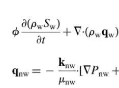
Assuming that the porous medium is nondeformable (constant porosity) and that cross-product permeability terms associated with the viscous drag tensor25 can be neglected, the general form of the two-fluid flow equations (without source–sink terms) is described by the two-fluid, volume-averaged momentum and continuity equations26
qw¼ ¹
kw
mw
·[=Pwþrwg] (1a) Table 1. Physical properties of fluids at 208C
Interfacial tension (N/m) Air–oil Oil–water Air–water
0.0681a
Soltrol 130 (Columbia) 0.0239a 0.0259a
Soltrol 220 (Lincoln) 0.0259a 0.036423
Viscosity (Ns/m2310¹3) Oil Air Water
0.0181 1.00
Soltrol 130 1.44
Soltrol 220 3.92
Density (kg/m3)
1.20 998
Soltrol 130 762
Soltrol 220 803
a
f](rwSw)
In eqns (1a), (1b), (1c) and (1d), the subscripts w and nw denote the wetting and non-wetting fluids, respectively; Pi
(i¼w,nw) denotes pressure (M L¹1T¹2); Si(i¼w,nw) is
the degree of fluid saturation relative to the porosity f
(volumetric fluid content vi¼fSi); qi is the flux density
vector (L/T); g is the gravitational acceleration vector;mi
andridenote dynamic viscosity (M L¹1T¹1) and density
(M L¹3), respectively; ki¼krik is the effective
permeabil-ity tensor (L2), where k is the intrinsic permeability (L2) and kri¼kri(Si) is the relative permeability.
Assuming that the porous media is nondeformable implies that
SwþSnw¼1 orvwþvnw¼f (2)
Assuming one-dimensional vertical flow and that the wet-ting fluid is incompressible, substitution of eqn (1a) into eqn (1b) yields
When replacing fluid pressures (Pwand Pnw) and capillary
pressure (Pc ¼Pnw¹Pw) with pressure head, defined by
transient flow of the wetting fluid is described by
Cw
the wetting fluid is compressible (e.g. air is the non-wetting fluid), substitution of eqn (1c) into eqn (1d) yields
](rnwvnw)
For air as the non-wetting fluid, it is furthermore assumed that its density is a linear function of the pressure head28, or
wherero,nwand ho are the reference density and pressure
head (at atmospheric pressure), respectively. The ratio
ro,nw/ho is defined as the compressibility l (l ¼ 1.24 3
10¹6g/cm4). Subsequently, using relationships eqns (4) and (7), and writing water potential in terms of pressure head27
yields the flow equation for the non-wetting fluid:
f¹vw
Eqns (5) and (8) can be solved simultaneously for the unknown pressure heads hwand hnw, and thus for hcas well.
The upper boundary condition at the top of the soil core (ztop) to be used in the inverse modeling of two-fluid flow is
described by a zero wetting fluid flux and by a sequence of imposed non-wetting fluid pressures, defined by Pnw(Tj), or
qw(ztop,t)¼0 (9a)
hnw(ztop,t)¼hnw(Tj)¼Pnw(Tj)
rH2Og
j¼1,2, …,M (9b)
where M is the total number of pressure steps used during time period Tj in the multi-step experiment. At the lower
boundary of the core (zbottom), the flux of the non-wetting
fluid is zero since the entry value of the ceramic plate for the non-wetting fluid is greater than any of the imposed pressures. The wetting fluid pressure at zbottomis determined
by the height of the wetting fluid in the burette, which is a function of time as the wetting fluid drains into the burette (Fig. 1), or
Finally, the initial condition for the multi-step method is given by the static pressure of each fluid at time t1:
hw(z,t1)¼hw(zbottom,t1)¹
where z is assumed positive upwards and z ¼ 0 at the bottom of the ceramic plate. hw(zbottom,t1) and hnw(ztop,t1)
denote the boundary pressure head values at the start of the transient outflow experiment.
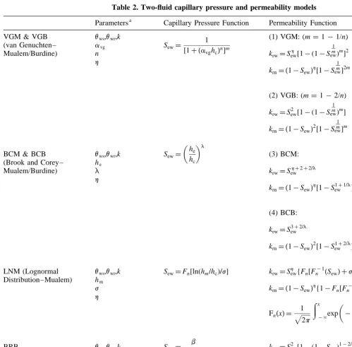
2.3 Constitutive relationships—parametric models
Parameter estimation requires the functional description of the capillary pressure–saturation, hc(Sw), and permeability
functions, ki(Sw), in eqns (5) and (8). The choice of a
Perhaps one of the most commonly used models of capil-lary pressure–saturation function is the van Genuchten29 equation (VG)
Sew¼[1þ(avghc) n]¹m
(12)
where Sew denotes the effective saturation of the wetting
fluid, Sew¼ ðvw¹vwrÞ/(vws¹vwr), wherevwsandvwrare the
saturated and residual wetting fluid saturation, respectively;
avgand n are fitting parameters, that are inversely
propor-tional to the non-wetting fluid entry pressure value and the width of pore-size distribution, respectively. In subsequent analysis, we assume that m¼1¹1/n, and that the effective saturation of the non-wetting fluid (Sen) is derived from Sen¼1¹Sew.
The Brooks and Corey (BC) model30is based on empiri-cal observations that log(Sew) is linearly related to log(hc),
yielding a power form of Sew(hc)
Sew¼(he=hc)l, hc.he (13a)
Sew¼1, hc#he (13b)
where he and l are characteristic soil parameters with l
characterizing the pore-size distribution and heequal to the
non-wetting fluid entry pressure. The VG model is asymp-totically equal to the BC model in the dry range when hc
becomes large, as then Sew<[(1/a)/hc]mn, such that 1/a¼ he and mn¼l.
The lognormal distribution (LN) model31,32 is based on the assumption that soils are represented by a lognormal pore-radius distribution yielding a two-parameter model for the capillary pressure–saturation function
Sew¼Fn distribution function that can also be calculated from Fn(x)¼1=2erfc(x=
2 p
). In eqn (14), the parameters hmand
j are physically based and are related to the geometric mean and variance of the pore-size distribution.
The Brutsaert (BR) capillary pressure–saturation func-tion33is of the form
Sew¼
b bþhgc
(15)
where b and g are fitting parameters characterizing the porous medium.
While the capillary pressure–saturation function can be considered a static soil property, the permeability function is a hydrodynamic property describing the ability of the soil to conduct a fluid. Capillary pressure–permeability prediction models were developed from conceptual models of flow in capillary tubes combined with pore-size distribution knowl-edge derived from the capillary pressure–saturation rela-tionship. Typical representations of this type of model
include Burdine4and Mualem34
Burdine(B): krw¼S
Combining the van Genuchten capillary pressure–satura-tion eqn (12) with the Mualem (VGM) model yields permeability functions as defined by 35
krw¼
Similarly, substituting eqn (13) into eqn (17) and integrat-ing yields the BCM formulation 34
krw¼Shþ
Similarly, the BCB model is derived by substituting eqn (13) into eqn (16) and integrating30
krw¼S
Comparison of eqns (18) and (19), indicates that the BCB model differs from the BCM model only by the tortuosity parameterh.
into eqn (16) and integrating to obtain36
Similarly, the LNM model is derived by substitution of eqn (14) into eqn (17) and integrating to obtain32
krw¼Shew Fn F
No closed-form Burdine or Mualem permeability models are available for the BR capillary pressure–saturation model eqn (15). However, through simplifying eqn (15), Brutsaert33obtained a closed form Burdine model (BRB)
krw¼S
Finally, combining the Gardner37equation
krw¼e¹ag hc
(24a)
with eqn (17) and usingh¼0, Russo21derived a capillary pressure–saturation relation (GD)
after which also the non-wetting permeabilitity relationship can also be derived (GDM)
krn¼ 1¹e
In subsequent analyses, for convenience in modeling and due to lack of information to the contrary, we set the h
value equal to 0.5 for both the wetting and non-wetting permeability expressions34, despite possible physical reasoning suggesting that h values for wetting and non-wetting fluids may differ38.
2.4 Numerical solution of governing equations and optimization method
The governing eqns (3) and (6), or eqns (5) and (8) if fully expressed in pressure head form, in combination with the boundary and initial conditions eqns (9), (10) and (11), with the constitutive relationships described in Table 2, deter-mine the mathematical model of the experimental system. No analytical solution is possible because of the nonlinear-ity of the constitutive functions. Therefore, we adapted the two-fluid flow numerical model of Dr J.L. Nieber,
University of Minnesota (personal communication) to simu-late the transient behavior of two-fluid phase flow as mea-sured in the multi-step outflow experiments. We used this numerical scheme, including the modified Picard lineariza-tion algorithm of the mixed-form governing equalineariza-tions and a lumped finite-element approximation39,28.
The inverse parameter estimation method is a nonlinear optimization problem, where a vector b containing the unknown parameters of the constitutive relationships is esti-mated by minimizing an objective function O(b), containing deviations between observed and predicted system response variables for the considered time period. For a given true predictive model (eqns (5) and (8)), formulation of the objective function (OF) using maximum likelihood (ML) considerations yields parameter estimates with non-zero values of the objective function being attributed to measurement errors40,12.
Using the notation v as the vector containing the elements of measured flow variables (capillary pressure head, out-flow) with the subscript m and s denoting measured and simulated values, respectively, the observation error is given by e ¼vm ¹vs(b), with the assumption that model
errors are zero. When observation errors are assumed to describe a multivariable normal distribution with zero-mean and covariance matrix V ¼ E(vm ¹ vs)(vm ¹vs)T,
the ML estimation results in the formulation of the negative log likelihood function, L45
L¼n
which after removing the constant terms leads to the objec-tive function, O(b), to be minimized:
O(b)¼eTV¹1e (26)
Thus, for a general covariance matrix V, eqn (26) repre-sents a general least squares problem, where the inverse of the error covariance matrix is the weighting matrix that includes measurement accuracy and correlation. In this study, we assume that the measurement errors of e are independent of each other and that their variances are pro-portional to the magnitudes of the mean values of particular measurements, so that V is a diagonal matrix12. In addition, weighting factors were chosen to be inversely proportional to their mean measured values of cumulative drainage (Q), capillary pressure head (hc) and initial water content
v(hc,1,t1), yielding a weighted least squares (WLS) problem
In eqn (27), the subscripts m and s denote measured and simulated values, respectively, and N, M and L refer to the number of observations of Q, hc andv, respectively. The
objective function, O(b), is normalized by the weighting factors:
initial volumetric wetting fluid content value corresponding with the initial capillary pressure head value (hc,1) at
hydraulic equilibrium before the first pressure step was applied and estimated from cumulative outflow after satura-tion. Weighting factorsqj,qkandqlwere arbitrarily set to
1, 1 and 15, respectively. The large value ofqlprovides a
disproportionally large weight tovm(hc,1,t1), thereby forcing Table 2. Two-fluid capillary pressure and permeability models
Parametersa Capillary Pressure Function Permeability Function VGM & VGB
the optimized capillary pressure–saturation curve to pass through this measured point of the capillary pressure curve. The objective of the optimization procedure is to deter-mine the parameter vector b that minimizes eqn (27). The objective function O(b) is a nonlinear function of b, so that minimization calculations must be carried out iteratively until pre-defined convergence criteria were satisfied. A commonly applied criterion is based on the relative decrease of RMS (root of mean squared residuals) value given by
RMS¼
O(b)
MþNþL
r
(30)
The Levenberg–Marquardt optimization algorithm41 was applied to minimize eqn (27) using the optimization pro-gram of Eching and Hopmans9, which was originally devel-oped by Kool et al.42, but was modified to interface with the two-fluid flow model.
The parametric models of Table 2 were evaluated based on: (1) comparison of their respective RMS values; (2) pos-teriori testing of the uniqueness of parameter sets; and (3) model simplicity (in terms of number of fitting parameters). Criteria that consider the number of fitting parameters include the Akaike information criterium (AIC) and the Bayesian information criterium (BIC), which are defined
by21,40
AIC¼N{ln(2p)þln[SSR=(N¹p)]þ1}þp (31)
and
BIC¼(AIC¹2p)þplnN (32)
where N and p are the total numbers of observation points and adjustable parameters, respectively, and SSR denotes the sum of squared residuals, numerically equal to O(b). The most parsimonious model minimizes both AIC and BIC, i.e. with their values for the considered fitting models being equal, the model with the least number of fitting parameters is the most acceptable. Hence, the criteria in eqns (31) and (32) penalize for additional fitting para-meters.
2.5 Scaling methodology
Scaling of interfacial surface tension values provides an additional means by which to evaluate the accuracy of the optimized capillary pressure–saturation functions. In addi-tion to a rigid porous media matrix, the Leverett scaling approach6 assumes that fluids are held in the porous matrix by capillary forces only. In this approach the dimen-sionless function, J(Sew) is introduced to describe the
simi-larity relationship between two arbitrary soil systems
J(Sew)¼ Pc,1
j1 k1
f1
12
¼Pc,2
j2 k2
f2
12
(33)
wherejand k denote interfacial tension and intrinsic per-meability, respectively. In eqn (33), (k/f)¹1/2 can be regarded as a microscopic length that depends on the pore geometry only. Therefore, for the same soil matrix with different fluid pairs 1 and 2, eqn (33) reduces to:
hc,2(Sew)¼
j2
j1
hc,1(Sew) (34)
Thus, using eqn (34), the capillary pressure–saturation relationship for a particular fluid pair (e.g. air–water) can be used to predict those for other fluid pairs using the appropriate interfacial tension values. Correct application
of eqn (34) further requires that: (i) the soil is completely water-wet; (ii) the oil phase is the intermediate wetting fluid between the water and air; and (iii) there is no fluid entrap-ment. It is also assumed that the contact angle is independent of fluid type, the veracity of which is under debate43.
The optimized capillary pressure hc(Sw) functions of air–
oil, and oil–water systems were scaled using the air–water system as a reference. Hence, scaled hc(Sw) curves for the
air–oil (ao) and oil–water (ow) systems were determined through multiplication of the optimized hcvalue byjaw/jao
and jaw/jow, respectively, based on the j values listed in
Table 1.
3 RESULTS AND DISCUSSION
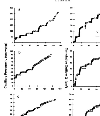
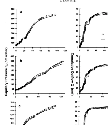
The inverse parameter estimation procedure was applied to multi-step outflow data for the three two-fluid pairs (air– water, air–oil, and oil–water) and both soils, and parameters were optimized for all seven capillary pressure–saturation and permeability relationships listed in Table 2. Figs 2 and 3 illustrate the comparison of measured with optimized cumu-lative outflow and capillary pressure heads for the air–water (aw), air–oil (ao), and oil–water (ow) systems of the Lincoln and Columbia soil, respectively, using the VGM constitutive relationships. These are examples of the type of agreement between optimized and measured values achieved with four of the constitutive functions, VGM, LNM, BRB, and GDM. Optimized simulations using the remaining three relationships (VGB, BCM, and BCB) fitted the multi-step data poorly, and are not shown. The sum of RMS values for each two-fluid flow system, consti-tutive model and soil are listed in Table 3. The relatively small RMS values in Table 3 for the VGM, LNM, BRB and GDM models, as compared to those for the VGB, BCM and BCB models, further supported our observations of the qual-ity of fit between measured and simulated results.
The parametric models considered here required six (GDM) or seven parameters. The choice of how many and which parameters to optimize was based on several considerations. First, it must be recognized that as the num-ber of parameters to be optimized increases, the parameter estimation procedure generally leads to better prediction of
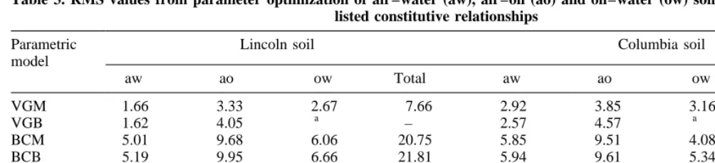
Table 3. RMS values from parameter optimization of air–water (aw), air–oil (ao) and oil–water (ow) soil systems for the seven listed constitutive relationships
Parametric model
Lincoln soil Columbia soil
aw ao ow Total aw ao ow Total
VGM 1.66 3.33 2.67 7.66 2.92 3.85 3.16 9.93
VGB 1.62 4.05 a – 2.57 4.57 a –
BCM 5.01 9.68 6.06 20.75 5.85 9.51 4.08 19.44
BCB 5.19 9.95 6.66 21.81 5.94 9.61 5.34 20.89
LNM 2.02 4.28 2.80 9.10 3.54 4.29 4.14 11.97
BRB 1.56 4.55 2.48 8.59 2.95 2.67 3.65 9.27
GDM 2.46 5.88 4.44 12.78 5.05 4.68 5.46 15.19
a
measured flow variables using these optimized parameters. However, this occurs at the expense of the uniqueness of the optimized solution and a corresponding increase in the uncertainty of the parameter estimates. Thus, it is preferred to minimize the total number of fitting parameters. If a parameter can be measured independently with relatively high accuracy, it should be fixed rather than obtained through optimization. Therefore, the saturated wetting-fluid content (vws) obtained experimentally for each soil
core from cumulative outflow and initial fluid saturation22 was fixed to measured values of 0.45 cm3cm¹3(Columbia) and 0.33 cm3cm¹3(Lincoln). To further reduce the number of optimizable parameters, we set h ¼ 0.534 for the permeability functions. Though the intrinsic permeability
(k) could be measured independently, we found that fixing
k overconstrained the permeability relationship such that its
shape was determined by only a single fitting parameter. Moreover, differences in pore geometry between the larger pores (defining soil structure) and soil matrix pores (defined by soil texture) resulting in bi-modal pore-size dis-tributions may preclude use of a intrinsic permeability value determined from measurements of K for a saturated soil2,44. Consequently, the constitutive relationships (Table 2) were estimated using four fitting parameters (k,vr, and two
addi-tional capillary pressure parameters), with the exception of the GDM model that is described by three fitting parameters (k,vrandag). Others
9,15
have demonstrated that this chosen set of fitting parameters are most sensitive to the
experimental data obtained from the multi-step outflow experiment when cumulative outflow measurements are supplemented with capillary pressure measurements.
Since the VGB model failed to converge for the oil–water system data of both soils, and the BC-type models (BCM and BCB) resulted in RMS values twice as large as that for the remaining models, we eliminated these three models from further evaluation. A possible reason for the poor pre-dictive behavior of the BC-type models in the multi-step outflow application is that experimental capillary pressures values were always larger than the non-wetting-fluid entry
pressure, thereby reducing the significance of the displacement pressure parameter of these models in the optimization. It was surprising to find that the GDM model, with only three fitted parameters is able to describe the soil’s capillary pressure and permeability relations almost as well as the other parametric models, which have one additional fitting parameter.
The uniqueness of the optimized parameter sets was tested using three different sets of initial parameter values. Initial parameter estimates were chosen to cover a wide range, but were somewhat constrained to preserve their physical meaning. For example, minimum values of both
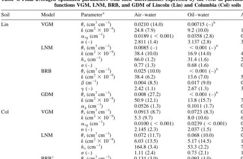
Table 4. Final averaged optimized parameters with their uncertainties expressed by the NSD in parentheses (%) for hydraulic functions VGM, LNM, BRB, and GDM of Lincoln (Lin) and Columbia (Col) soils
Soil Model Parametera Air–water Oil–water Air–oil
Lin VGM vr(cm3cm¹3) 0.0210 (14.0) 0.00715 (–)b ,0.001 (–)
k (cm2310¹9
) 24.8 (7.9) 9.2 (10.0) 10.9 (17.0)
avg(cm¹1) 0.0189 (,0.001) 0.0358 (2.8) 0.0529 (1.9)
n (–) 2.811 (1.4) 3.137 (2.8) 3.002 (2.5)
LNM vr(cm
3
cm¹3
) 0.0085 (–) ,0.001 (–)b ,0.001 (–)b
k (cm2310¹9
) 38.4 (10.0) 16.9 (14.0) 4.2 (14.8)
ho(cm
¹1
) 66.0 (1.2) 31.4 (1.6) 24.5 (0.85)
j(–) 0.77 (1.3) 0.68 (1.6) 0.382 (3.2)
BRB vr(cm3cm¹3) 0.025 (10.0) ,0.001 (–)b ,0.001 (–)b
k (cm2310¹9) 38.4 (6.2) 13.6 (7.0) 5.0 (14.0)
b(m¹1) 0.004 (8.5) 0.017 (9.0) 0.002 (47.0)
g(–) 2.42 (1.1) 2.67 (1.3) 3.44 (4.7)
GDM vr(cm3cm¹3) 0.008 (27.2) ,0.001 (–)b ,0.001 (–)b
k (cm2310¹9) 50.9 (12.1) 13.8 (15.7) 7.2 (20.6) ag(cm¹1) 0.0526 (1.3) 0.1011 (1.7) 0.1450 (3.8)
Col VGM vr(cm3cm¹3) 0.0913 (8.7) 0.0723 (8.3) 0.0613 (9.5)
k (cm2310¹9
) 5.3 (9.7) 8.0 (10.6) 6.2 (10.4)
avg(cm¹1) 0.0100 (,0.001) 0.0239 (,0.001) 0.0253 (,0.001)
n (–) 2.145 (2.3) 2.037 (1.5) 2.694 (1.8)
LNM vr(cm3cm¹3) 0.072 (11.7) 0.068 (10.0) 0.083 (8.8)
k (cm2310¹9
) 6.03 (13.5) 5.17 (14.5) 19.6 (19.0)
ho(cm¹ 1
) 164.8 (3.4) 53.3 (2.2) 72.8 (3.5)
j(–) 1.11 (2.4) 0.73 (2.1) 1.03 (2.2)
BRBc vr(cm
3
cm¹3) 0.134 (3.0) 0.093 (4.0) 0.13 (3.4)
k (cm2310¹9) 27.8 (17.2) 9.7 (9.3) 81.6 (24.0)
b(m¹1) 0.0031 (18.1) 0.0032 (18.2) 0.02 (17.5)
g(–) 2.120 (1.8) 2.68 (1.3) 2.1 (2.2)
GDM vr(cm3cm¹3) 0.135 (3.4) 0.066 (8.3) 0.145 (2.9)
k (cm2310¹9) 10.3 (17.1) 6.4 (15.1) 55.1 (27.0) ag(cm¹1) 0.0209 (1.8) 0.0661 (2.4) 0.0485 (3.3) av
sis fixed for both soils;vs¼0.33 cm3cm¹3for Lincoln and 0.45 cm3cm¹3for Columbia soil. b
Optimized parameter is close to zero, thereby providing a meaningless NSD value.
c
Not all optimizations converged for air–oil system.
Table 5. AIC and BIC values for selected models
Soil Model Air–water Air–oil Oil–water
AIC BIC AIC BIC AIC BIC
Lincoln VGM 1773 1790 1758 1773 1647 1663
LNM 1929 1943 1841 1856 1688 1703
BRB 1717 1734 1876 1891 1550 1565
GDM 2136 2149 2039 2050 1960 1972
Columbia VGM 1218 1232 1265 1278 1246 1260
LNM 1311 1325 1311 1325 1377 1391
BRB 1215 1229 1136 1150 1320 1334
permeability and residual water content were always posi-tive. Final parameter values are listed in Table 4. The final parameter set was taken as that having the minimum RMS value, or was computed from mean parameter values if the optimized parameter sets had similar minimum RMS values. The uncertainty in the optimized parameter values in Table 4 is expressed by the normalized standard deviate (NSD), which was calculated from (ji/bi)3100%, whereji
is the standard deviation of parameter bias estimated from
the parameter covariance matrix12. Using this type of expression, the uncertainties of the parameters can be eval-uated by direct comparison of NSD values. Larger NSD values indicate increasing parameter uncertainty and decreasing parameter sensitivity. In general, it can be con-cluded from the results in Table 4 that k has the largest uncertainty and smallest sensitivity. Consequently, although
k is a function of the porous medium only, optimized k
values vary widely between fluid pair and hydraulic func-tion type. Finally we point out that not all optimizafunc-tions converged for the BRB model.
In addition to visual comparison of predicted and measured cumulative outflow and capillary pressure head values, and evaluation of RMS and NSD values, a third approach to discriminate between parametric models is by comparison of the respective AIC and BIC values, accepting those models with minimum AIC or BIC values. These values are listed in Table 5 for the VGM, LNM, BRB, and GDM models. Although the GDM model has one para-meter less than all other models, AIC and BIC values are still largest because of its high RMS values (Table 3). The advantage of the reduced number of fitting parameters of the GDM model is partly offset by the large number of data
values. Hence we conclude a slight advantage for the VGM, LNM and BRB models.
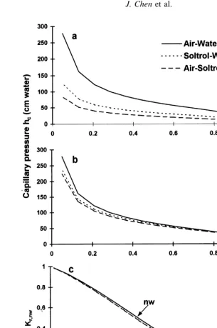
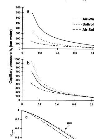
Finally, as a means of testing the modified Leverett scal-ing relationships usscal-ing the optimized parameters of the VGM model, we included the scaled capillary pressure functions in Fig. 4 (Lincoln) and Fig. 5 (Columbia), together with the optimized capillary pressure–saturation and per-meability curves. The capillary pressure–saturation curve of the air–water system was used in applying the scaling
relationships of eqn (34). The scaled curves match extre-mely well at high saturations. Deviations at low satura-tions are similar to that observed by Demond and Roberts43, who suggested that such deviations were caused by limitations of the surface tension scaling approach associated with uncertainties of the contact angle value. Similar results comparing scaled relationships and optimized relationships were obtained for the remaining constitutive models. For the modified Leverett scaling theory to apply, the avg values (VGM model) of a fluid
pair must be inversely proportional to the corresponding interfacial tension values. Table 6 summarizes the avg
andjratios of the respective fluid pairs, and indicates that both ratios are almost identical, thereby further validating the parameter estimation approach for two-fluid outflow experiments.
Fig. 5. Optimized constitutive functions (VGM) of Columbia soil corresponding to the parameters listed in Table 4: (a) individual capillary pressure–saturation functions; (b) scaled capillary pressure–saturation functions; and (c) relative permeability functions.
Table 6. Interfacial tension andavgratios for oil–water and
air–oil systems relative to air–water system
jow/jaw aaw/aow jao/jaw aaw/aao
Columbia 0.38 0.42 0.35 0.40
4 CONCLUSIONS
The soil capillary pressure–saturation and permeability– saturation functions are important for subsurface flow modeling applications. We demonstrate the feasibility of using the inverse parameter estimation method for two-fluid flow systems in multi-step outflow experiments. Though it is impossible to remove all inherent uncertainty stemming from the nonlinearity and complexity of fluid transport in soil systems, a posteriori analysis of the inverse problem indicated that the inverse parameter estimation of the constitutive functions from transient multi-step outflow experimental data for two-fluid systems is a well-posed pro-blem. The good agreement between the experimentally measured and optimally simulated system responses indi-cates that the inversely estimated constitutive relationships do indeed characterize the two porous systems investigated. Model discrimination for inverse parameter estimation is evaluated based on RMS and AIC and BIC values, para-meter uniqueness, model convergence, and comparison of the scaled relationships of the optimized functions. Overall, both the commonly applied VGM and the physically-based LNM models show high estimation accuracy and low RMS values, while yielding similar AIC and BIC values. Although the BRB model yielded low RMS values, it showed convergence problems for the oil–water systems, similar to the VGB model. Despite the GDM model having only three fitting parameters, AIC and BIC values were larger than any of the three other models, whereas the result-ing RMS values were only slightly larger than those for the three other acceptable models. It appears that the VGM, LNM, BRM, and GDM models are equally applicable, with slight individual nuances, in the inverse parameter estimation of multi-step outflow data. The BC-type models showed a poor performance, likely caused by the absence of measured non-wetting-fluid entry values in the objective function. Further evaluation of the optimum model may depend on the considered soils and fluids, and experimental conditions. A relatively broad range of selected model options also indicates the flexibility and robustness of the presented inverse parameter estimation approach. Advan-tages inherent to the parameter estimation method include that the measurements are simple and accurate, the simulta-neous estimation of capillary pressure and permeability functions for the same soil sample, and the consistency of the application in computer modeling. In summary, we con-clude that the multi-step outflow method is an accurate and efficient method for determination of two-fluid flow capil-lary pressure–saturation and permeability functions.
ACKNOWLEDGEMENTS
This study was financed by the EPA (RFA 93-G4) under cooperative agreement No. CR-822204. We are especially grateful to Dr John L. Nieber at the University of Minnesota,
for supplying us with his transient one-dimensional two-phase flow code that we adapted for our study.
REFERENCES
1. Dane, J.H., Oostrom, M. and Missildine, B.C. An improved method for the determination of capillary pressure–saturation curves involving TCE, water and air. J. Contam. Hydro., 1992, 11, 69–81.
2. Demond, A.H. and Roberts, P.V. Estimation of two-phase relative permeability relationships for organic liquid con-taminants. Water Resour. Research, 1993, 29, 1081–1090. 3. Klute, A. and Dirksen, C., Conductivities and diffusivities of
unsaturated soils. In Methods of Soil Analysis, Agron. Monogr. 9, Part 1, 2nd edn, ed. A. Klute. ASA and SSSA, Madison WI 53711, 1986, pp. 687–734.
4. Burdine, N.T. Relative permeability calculations from pore size distribution data. Petroleum Trans. Am. Inst. Mining Eng., 1953, 198, 71–77.
5. Mualem, Y. and Dagan, G. Hydraulic conductivity of soils: Unified approach to the statistical models. Soil Sci. Soc. Amer. J., 1978, 42, 392–395.
6. Leverett, M.C. Capillary behavior in porous solids. Trans. AIME, 1941, 142, 152–169.
7. Miller, E.E. and Miller, R.D. Physical theory for capillary flow phenomena. Journal of Applied Physics, 1956, 27, 324–332. 8. Dane, J.H. and Hruska, D. In-situ determination of soil
hydraulic properties during drainage. Soil Sci. Soc. Am. J., 1983, 47, 619–624.
9. Eching, S.O. and Hopmans, J.W. Optimization of hydraulic functions from transient outflow and soil water pressure data. Soil Sci. Soc. Am. J., 1993, 57, 1167–1175.
10. Eching, S.O., Hopmans, J.W. and Wendroth, O. Unsaturated hydraulic conductivity from transient multistep outflow and soil water pressure data. Soil Sci. Soc. Am. J., 1994, 58, 687–695.
11. Hornung, U., Identification of nonlinear soil physical para-meters from an output–input experiment, in numerical treat-ment of inverse problems in differential and integral equations, ed. P. Deuflhard and E. Hairer. Birkhauser, Boston MA, 1983, pp. 227–237.
12. Kool, J.B. and Parker, J.C. Analysis of the inverse problem for transient unsaturated flow. Water Resources Research, 1988, 24, 817–830.
13. Parker, J.C., Kool, J.B. and Van Genuchten, M.Th. Determin-ing soil hydraulic properties from onestep outflow experi-ments by parameter estimation: II. Experimental studies. Soil Sci. Soc. Amer. J., 1985, 49, 1354–1359.
14. Russo, D., Bresler, E., Shani, U. and Parker, J.C. Analysis of infiltration events in relation to determining soil hydraulic properties by inverse problem methodology. Water Resources Research, 1991, 27, 1361–1373.
15. Toorman, A.F., Wierenga, P.J. and Hills, R.G. Parameter estimation of hydraulic properties from one-step outflow data. Water Resources Research, 1992, 28, 3021–3028. 16. Zachmann, D.W., Duchateau, P.C. and Klute, A. The calibration
of the Richards’ flow equation for a draining column by para-meter identification. Soil Sci. Soc. Am. J., 1981, 45, 1012–1015. 17. Zachmann, D.W., Duchateau, P.C. and Klute, A. Simulta-neous approximation of water capacity and soil hydraulic conductivity by parameter identification. Soil Sci., 1982, 134, 157–163.
19. Gardner, W.R. Calculation of capillary conductivity from pressure plate outflow data. Soil Sci. Soc. Amer. Proc., 1956, 20, 317–320.
20. van Dam, J.C., Stricker, J.N.M. and Droogers, P. Inverse method to determine soil hydraulic functions from multistep outflow experiments. Soil Sci. Soc., Am. J., 1994, 58, 647–652.
21. Russo, D. Determining soil hydraulic properties by parameter estimation: on the selection of a model for the hydraulic properties. Water Resources Research, 1988, 24, 453–459. 22. Liu, Y.P., Hopmans, J.W., Grismer, M.E. and Chen, J.Y.
Direct estimation of air–oil and oil–water capillary pressure and permeability relations from multi-step outflow experi-ments. J. Contam. Hydrology, 1998, 32, 21–42.
23. Schroth, M.H., Istok, J.D., Ahearn, S.J. and Selker, J.S. Geo-metry and position of light nonaqueous phase liquid lenses in water-wetted porous media. J. Contam. Hydrol., 1995, 19, 269–287.
24. Hopmans, J.W., Vogel, T. and Koblik, P.D. X-ray tomogra-phy of soil water distribution in one-step outflow experi-ments. Soil Sci. Soc. Am. J., 1992, 56, 355–362.
25. Whitaker, S.A. The closure problem for two-phase flow in homogeneous porous media. Chemical Engineering Science, 1994, 49, 765–780.
26. Bear, J., Dynamics of fluids in porous media. Dover Publica-tions, New York, 1972.
27. Touma, J. and Vauclin, M. Experimental and numerical ana-lysis of two-phase infiltration in a partially saturated soil. Tranport in Porous Media, 1986, 1, 27–55.
28. Celia, M.A. and Binning, P. A mass conservative numerical solution for two-phase flow in porous media with application to unsaturated flow. Water Resources Research, 1992, 28, 2819–2828.
29. van Genuchten, M.Th. A closed-form equation for predicting the hydraulic conductivity of unsaturated soils. Soil Sci. Soc. Am. J., 1980, 44, 892–898.
30. Brooks, R.H. and Corey, A.T., Hydraulic properties of porous media. Colorado Univ., Hydrology paper No. 3, 1964. 31. Kosugi, K. Three-parameter lognormal distribution model for soil water retention. Water Resour. Research, 1994, 30, 891–901.
32. Kosugi, K. Lognormal distribution model for unsaturated soil hydraulic properties. Water Resources Research, 1996, 32, 2697–2703.
33. Brutsaert, W. Some methods of calculating unsaturated per-meability. Trans. ASAE, 1967, 10, 400–404.
34. Mualem, Y. A new model for predicting the hydraulic con-ductivity of unsaturated porous media. Water Resources Research, 1976, 12, 513–522.
35. Luckner, L., van Genuchten, M.Th. and Nielsen, D.R. A consistent set of parametric models for the two-phase flow of immiscible fluids in the subsurface. Water Resources Research, 1989, 25, 2187–2193.
36. van Genuchten, M.Th., Calculating the unsaturated hydraulic conductivity with a new closed-form analytical model, Res. Rep. 78-WR-08, Dept. of Civil Eng., Princeton Univ., Princeton NJ, 1978.
37. Gardner, W.R. Some steady state solutions of unsaturated moisture flow equations with application to evaporation from water table. Soil Sci., 1958, 85, 228–232.
38. Finsterle, S. and Pruess, K. Solving the estimation-identifica-tion problem in two phase flow modeling. Water Resources Research, 1995, 31, 913–924.
39. Celia, M.A., Bouloutas, E.T. and Zarba, R.L. A general mass-conservative numerical solution for the unsaturated flow equation. Water Resources Research, 1990, 26, 1483–1496.
40. Carrera, J. and Neuman, S.P. Estimation of aquifer para-meters under transient and steady state conditions: 1. Max-imum likelihood incorporating prior information. Water Resources Research, 1986, 22, 199–210.
41. More, J.J., The Levenberg–Marquardt algorithm: Implemen-tation and theory. In Lecture Notes in Mathematics, 630, ed. G.A. Watson. Springer-Verlag, New York, 1977.
42. Kool, J.B., Parker, J.C., and van Genuchten, M. Th., ONE-STEP: A nonlinear parameter estimation program for evalu-ating soil hydraulic properties from one-step outflow experiments. Virginia Agricultural Experiment Station, Bulletin 85-3, 1985.
43. Demond, A.H. and Roberts, P.V. Effect of interfacial forces on two-phase capillary pressure–saturation relationships. Water Resour. Research, 1991, 27, 423–437.
44. Simunek, J. and van Genuchten, M.Th. Parameter estimation of soil hydraulic properties from the tension disc infiltrometer experiment by numerical inversion. Water Resources Research, 1996, 32, 2683–2696.