ORIENTATION SPECTRUM ALGORITHM DEVELOPMENT
S. A. Brianskiya, S. V. Sidyakina, Yu. V. Viziltera,∗
aThe Federal State Unitary Enterprise ”State Research Institute of Aviation System”, Russia, Moscow - (sbrianskiy, sersid, viz)@gosniias.ru
KEY WORDS:Shape Analysis, Mathematical Morphology, Maragos Pattern Spectra, Continuous Skeletons, Disc Structuring Ele-ment, Orientation Spectrum
ABSTRACT:
A morphological orientation spectra is proposed. This spectrum describes basic directions of shape parts. Fast discrete-continuous algorithm for computing orientation spectrum is presented. It is based on usage of continuous skeleton that is constructed from polygonal shape contour. A definition for disc orientation map is given. Comparison experiments for binary shapes with the usage of orientation spectra are carried out. Cyclic shift and EMD-L1distance are used for spectra comparison. The obtained results indicate that the aggregation of the thickness spectra with orientation spectra increases the quality of inter-class recognition.
1. INTRODUCTION
In the field of computer vision, many approaches exist to the problem of description and analysis of the 2D shapes. Among them, pure analytical method or methods based on analytical so-lutions have an advantage. Such analytical methods are often very fast and allow to build more precise and compact descrip-tors then fully discrete methods. For example, in paper (Mestet-skiy, 2009) and (Masalovitch, 2009) computational effective al-gorithms were proposed for constructing continuous skeletons of 2D (flat) polygonal shapes. Continuous skeletons are infor-mative, but unstable descriptors. That is why, it is reasonable to use morphological pattern spectrum (Maragos, 1989) that is more stable (Sidyakin, 2013). Connection between various skele-tal representation (Mestetskiy, 2009) and a morphological pattern spectrum (Maragos, 1989) is also well-known. Morphological discrete-continuous morphological pattern spectrum (Sidyakin, 2013) with a disc structuring element (SE) can be calculated us-ing continuous skeleton and radial function (Mestetskiy, 2009) and (Masalovitch, 2009). This spectrum allows us to characterize the local thickness of shape parts, but tells us nothing about the ”orientation” of these parts. To solve this ”orientation” problem, we could use elliptical SE and existing efficient algorithm (Serra, 1982), but real accounting of all possible ellipse parameters com-binations reduces efficiency of elliptical discrete-continuous mor-phological pattern spectrum algorithm (Serra, 1982).
In this paper, we propose more simple and effective solution then the elliptic one in (Serra, 1982), which allows us to extract the in-formation about orientation of shape parts. Its core idea is to use the orientation of continuous skeleton bones and build one addi-tional discrete orientation accumulator a la algorithm (Sidyakin, 2013). Thus, the presented approach utilize the robustness and efficiency of continuous skeleton to build the orientation pattern spectra.
The remaining part of the paper is organized as follows. In sec-tion 2, theoretical concepts of morphological pattern spectrum and thickness map is given. In Section 3, the review of the re-lated pattern spectrum algorithms that are based on continuous skeletons are brought down. The proposed approach is presented in section 4. In section 5, we present the experimental results conducted on standard shape datasets. The comparative analysis
∗Corresponding author
with the existing similar disc spectrum approach is also presented in this section. The conclusion is given in section 6.
2. MORPHOLOGICAL PATTERN SPECTRUM
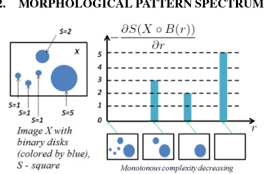
Figure 1: The morphological pattern spectrum of objects in the image X with disc SE and the stages of its morphological pro-cessing.
The original idea of pattern spectrum proposed by Maragos (Mara-gos, 1989) is based on Serra’s Mathematical morphology filters (opening/closing). More formally, letXbe the given binary im-age (pattern). LetB be the structuring element with (0,0) as the origin on the 2D object planeP. The parametrically scal-able structuring elementB(r)cab be defined asB(r)={rb|b∈
B}, r ≥0, b= (xb, yb) ∈ P. LetX ⊆P andB ⊆P, the morphological pattern spectrum(PS) ofXis defined as
P S(r) =−∂S(X∂r◦B(r)), r≥0 (1)
P S(−r) = ∂S(X•B(r))
∂r , r >0 (2)
whereS(X)=k X kL1, is the area of X, P S(r) - the
ri≥0
In the paper (Sidyakin, 2013), the new definition for pattern spec-trum with disc SE was given based on disc thickness maps.
LetF be a binary figure which fully fits on the frameK :F ⊆
K. DenoteFC(K)=K\F, thebackgroundof figureF on the frameK. Then the binary image, that correspond to the figureF, is defined as:
fF(x, y) =
(
1,ifp= (x, y)∈F;
0,ifp= (x, y)∈FC(K). (5)
Figure 2: Left: thickness map for foreground; Right: thickness map for background.
LetB(q, r)be a translatable flat disc with the center at the point q=(x, y)=B(q,0)and the scale parameterr. Definition 1. Thick-ness mapTB(fF)of a binary image fF(x, y) with disc struc-turing elementB(q, r)is real-valued image defined on the frame K, with each point representing the maximum size of its cover-ing disc structurcover-ing element fully inscribed in the figure shapeF. For the background of figureF, the value of the scale parameter is negative, as shown in fig. 2.
TB(fF) =
In particular, it was also proven in (Sidyakin, 2013) that discrete Maragos pattern spectrum with disc structuring element is a his-togram of discrete disc thickness map. The proposed disc thick-ness map made possible the creation of precise fast disc pattern spectrum computation algorithm. This algorithm is briefly de-scribed in the next section.
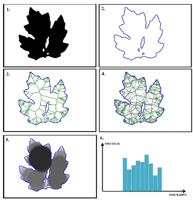
Figure 3: Discrete-continuous morphological pattern spectrum algorithm for disc SE. Steps from 1 to 6 shown. 1. 2D Shape; 2. Polygon; 3. Continuous skeleton; 4. Continuous skeleton and skeleton radial function; 5. Thickness map (as gray scale image). 6. Disc Spectrum as 1D histogram.
2.1 Fast Disc Algorithm For Pattern Spectra Construction
Fast Discrete-continuous disc spectrum algorithm (Sidyakin, 2013) sequentially goes through points of rasterized representation of continuous skeleton bones and accumulate (collect) point’s votes in cells (pixels) of the thickness accumulator. Vote value at the point is equal to the radial function value (radius of maximum inscribed empty circle with the center at this point) at the current skeleton bone’s point. Accumulation process of vote’s values in one cell is to choose maximum value between new vote value and vote value recorded before in this cell. Thickness map is a thickness accumulator filled with votes. As a result, values of the maximum inscribed empty discs are recorded in the cells (pix-els) of the thickness map and there is a connection link between points (pixels) of the shape and skeleton points, which are the centers of the maximum inscribed empty discs. The histogram of thickness map represents discrete disc spectrum. Fig. 3 shows the main steps of the described approach. Further the described technic was generalized for elliptical spectra (section 2.2.).
2.2 Elliptical Algorithm For Pattern Spectra Construction
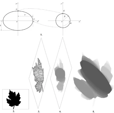
Figure 4: Basic ideas for pattern spectrum algorithm construction with fixed elliptical SE. The most important steps are shown. 1. Equi-affine transformation elliptical SE to disc SE; 2. Original 2D Shape; 3. Disc skeleton of equi-affine transformed polygonal shape; 4. Disc thickness map of transformed shape; 5. Elliptical thickness map obtained from disc thickness map by equi-affine transformation of disc SE to elliptical SE.
spectrum algorithm is deprived of this drawback and allows to take into account all the orientations presented in the figure.
3. ORIENTATION SPECTRUM ALGORITHM
To get started with orientation spectrum of 2D shapes, let’s de-fine the orientation property for all skeleton points. One possible definition of the orientation of the point is the tangent angle at this point to the skeleton. If the skeleton point is the node point (fig. 6) - this is a special case, and we assume that the orientation of the point is the tangent angle at this point to the skeleton bone with the maximum average thickness. If there are several bones of equal average thickness, we assume that there is no orientation at this node point.
Thus, 2D function (radial function, orientation) is given at all points of the skeleton. Therefore, maximum inscribed circles de-scribe the local thickness of shape that is elongated in a certain direction (have certain orientation). This orientation is assigned to the skeleton points.
Definition 2. Orientation map - 2D function, that is defined on the image. This 2D function has the value at each point, that is equal to the orientation of the bone to which the maximum empty disk of the maximum area, covering this point, belongs. So, Definition 2 is very similar to Definition 1.
Definition 3. Orientations spectrum is a histogram of orientation map.
Overall, the algorithm to obtain a morphological orientation pat-tern spectrum is presented below.
(a) Compute continuous polygonal representation (fig. 8.2) of binary figure (fig. 8.1)F(Mestetskiy, 2009).
Figure 5: Elliptical thickness maps for arbitrary (not fixed) ellip-tical SE. It is possible to build them based on discrete-continuous morphological pattern spectrum algorithm for fixed elliptical SE, but to do it fairly effectively we need to use a finite set of allowed ellipse parameters.
Figure 6: Continuous Skeleton of the polygonal figure. Site-points, site-segments, node-points are shown.
(b) Analytically calculate the continuous skeleton representation SR(F)(fig. 8.3) of the continuous polygonal figureF (all skeleton bones and radial function for these bones)(Masalovitch, 2007).
(c) Create a two-dimensional thickness accumulator and initial-ize all his elements with zeros. Create a two-dimensional orientation accumulator and initialize all his elements with zeros.
(d) Select a continuous bone (parabolical or line bone) from a list of skeleton bones. If the list is empty, go to (h).
(e) Compute discrete representation of the continuous bone with the help of Bresenham algorithm (Zingl, 2012) and form a set of points{pi(xi, yi, ri)}, defined by the coordinates(xi, yi) of the center and the radiusriof relevant maximum empty circles computed with the following equations (Mestetskiy, 2010):
- in the case of two site-segments we have a corresponding linear bone, that is described by the 1-st order Bezier curve:
V(t) =V0(1−t) +V1t
Figure 7: Orientation map construction for ”common red point”. Orientation map is build based on thickness map. b(rb, ob)- big maximum disc with center in point b, radiusrb and orientation ob.s(rs, os)- small maximum disc with center in point s, radius rsand orientationos.
whereV0, V1 - end points of linear bone,r0, r1- maximum inscribed discs’ radii that correspond to end points,t- curve parameter,t∈[0. . .1];
- in the case of site-segments and site-point, we have a cor-responding parabolical bone, that is described by the 2-nd order Bezier curve:
whereV0, V2- end points of parabolical bone,r0, r2- max-imum inscribed discs’ radii that correspond to end points, B1, B2 - end points of site-segment, t - curve parameter, t∈[0. . .1];
- in the case of two site-points we have a corresponding lin-ear bone, that is described by the 2-nd order rational Bezier curve:
whereV0, V2 - end points of linear bone,r0, r2- maximum inscribed discs’ radii that correspond to end points,t- curve parameter,t∈[0. . .1],ω1- weight coefficient,r1- control disk radius, x1 - control vertex on the abscissa axis. The system of equations (10) is solved To determiner1andx1:
(
r0r1−x0x1=c2
r2r1−x2x1=c2 (10)
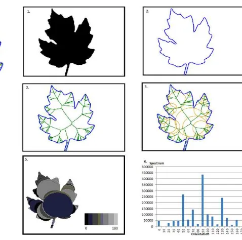
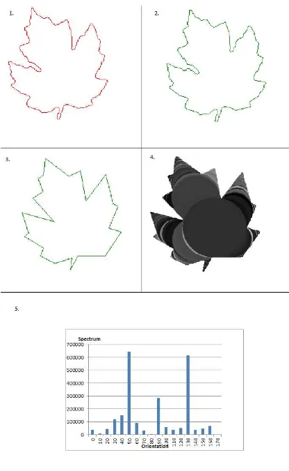
Figure 8: Creation of orientation pattern spectrum for disc SE. Steps from 1 to 6 shown. 1. 2D Shape; 2. Polygon; 3. Continuous skeleton; 4. Continuous skeleton and skeleton radial function; 5. Orientation map (orientation coded in color). 6. Orientation Spectrum as 1D histogram.
wherec- half of the distance between site-points. The system of equations (11) is solved to determineω1:
ω1= λ1
(f) Construct discrete thickness map and orientation map in ac-cumulators. The following logic is applied: bigger maxi-mum circles cover smaller maximaxi-mum circles. So, for current bone pointpiconstruct a filled maximum circle of the radius riin the accumulator with the help of Bresenham algorithm for discrete circle representation (fig. 8.4). When filling the circle with the value of radiusriin the corresponding accu-mulator elements, the following condition is checked: ifriis bigger than the current accumulator element value, storerito the current thickness accumulator element and orientationoi of the current disc to the current orientation accumulator el-ement, otherwise leave accumulators’ elements without any changes. Ifriis equal torj, chooseobased on average bone thickness. Return to step (d).
(g) Collect one-dimensional histogram (orientation spectrum)(fig. 8.6) or two-dimensional histogram (2D thickness and orien-tation spectrum) (fig. 7). Both ”orienorien-tation” based spectra can be used for shape comparison.
Figure 9: Polygonal contour of the shape: 1. Original polygonal contour; 2. Regularized contour with small regularization coeffi-cient; 3. Regularized contour with big regularization coefficoeffi-cient; 4. Orientation map (orientation coded in color); 5. Orientation spectrum of regularized shape.
(i) Normalize morphological orientation pattern spectrum: the sum of all spectrum bins should be equal to one.
To increase stability of the proposed descriptor it is recommended to regularize polygonal contour of the shape (fig. 9)(Sidyakin, 2013).
Adjustable parameter of this algorithm is the orientation sampling step. This parameter determines the sensitivity of the spectrum to the variety of orientations presented in the shape. 10 degrees step was chosen for the experiments.
4. EXPERIMENTS
In this section, we present the experimental results conducted on the standard shape dataset Kimia-216. The Kimia-216 shape dataset consists of 18 classes with 12 samples in each class. Ex-amples of objects of different classes are shown (fig. 10). All shapes (presented in images) in this dataset were transformed to the same shape-area-based scale (i.e, the scale is estimated such that the area of all shapes became equal 215140 pixels) and then all the images were bounded to the same image size (height = 507 pixels and width = 467 pixels). The comparison of shapes through the comparison of orientation spectra is performed by
Figure 10: Examples of classes dataset Kimia-216.
Figure 11: Average precision when comparing spectra with EMD-L1.
sequential cyclic shift. EMD-L1comparison of the shifted orien-tation spectra is applied on each shift step. The minimum EMD-L1value between all shift steps is taken. The performance of the proposed approach is demonstrated through top-raverage class precision for therclosest matching shapes (r = 11for Kimia-216). Below comparative results are shown for disc thickness spectra, for the proposed orientation spectra and for combination of 2D thickness/orientation spectra. The average time of compar-ison of two shapes by orientation spectra in Kimia-216 takes 18 ms.
Fig. 11 shows average class precision that was obtained by using thickness spectra and orientation spectra respectively. It is clear to see that in some cases orientation spectrum performs better than thickness spectrum. The thickness spectrum shows better results than orientation spectrum for the first three request images (fig. 12). For the last three request images, we have the opposite situation (fig. 13).
The experiment, when thickness spectra and orientation spectra were applied consequentially, was conducted. Orientation spectra was built for the reduced set of figures (24 images), these figure shapes were selected by thickness spectra. Average precision is shown on fig. 14.
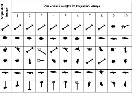
EMD-Figure 12: Top closest shapes for the requested shape. Thickness spectrum was used.
Figure 13: Top closest shapes for the requested shape. Orienta-tion spectrum was used.
L1comparison is stable to small deformations of flexible objects, to rotation and to slight noise effects at the borders of the shapes.
5. CONCLUSION
A morphological orientation spectra is proposed. This orienta-tion spectrum describes basic direcorienta-tions of shape parts in contrast to thickness spectrum. Orientation spectrum can be calculated much faster than elliptical spectrum with arbitrary elliptical SE. This descriptor is invariant to shift of a figure in the frame and can be also applied to the analysis of almost non flexible figures, parts of which can slightly change their directions. Fast discrete-continuous algorithm for computing orientation spectrum is pre-sented. It is based on usage of continuous skeleton that is con-structed from polygonal shape contour. A definition for disc ori-entation map is given. Comparison experiments for binary shapes with the usage of orientation spectra are carried out. Cyclic shift and EMD-L1 distance are used for spectra comparison. Cyclic shift helps to make comparison rotation invariant. The obtained results indicate that the aggregation of the thickness spectra with orientation spectra increases the quality of inter-class recognition. Proposed spectrum can also be used for shape segmentation into regions of different orientation and/or thickness.
Figure 14: Average precision for thickness spectra and thick-ness/orientation spectra.
REFERENCES
Maragos, P., 1989. Pattern Spectrum, Multiscale Shape Repre-sentation. In: Pattern Analysis and Machine Intelligence, IEEE Transactions on., Vol. 11, Issue 7, pp. 701-716.
Masalovitch, A., Mestetskiy L., 2007. Usage of continuous skele-tal image representation for document images de-warping. In: 2nd International Workshop on Camera-Based Document Analy-sis and Recognition, Curitiba, Brazil.
Mestetskiy, L. M., 2008. Continuous morphology of binary im-ages: figures, skeletons, circulars. Moscow, Russia, p. 288.
Mestetskiy, L.M. 2010. Skeleton of polygonal figure - represen-tation by planar linear graph // Proceedings of the 20th Interna-tional Conference on Computer Graphics and Vision, Graphicon 2010, St. Petersburg, pp. 222-229
Serra, J., 1982. Image Analysis and Mathematical Morphology. Academic Press, London, England, p. 610.
Sidyakin, S.V., 2013. Morphological pattern spectra algorithm development for digital image and video sequences analysis. PhD Thesis, Institution of Russian Academy of Sciences Dorodnicyn Computing Centre of RAS (CC RAS), Moscow, Russia.
Sidyakin, S.V., Vizilter Yu.V., 1989. Morphological shape de-scriptors of binary images based on elliptical structuring elements. In:Computer Optis, Samara, Russia, Vol. 38, Issue 3. pp. 511-520.