ITERATIVE DETERMINATION OF CAMERA POSE FROM LINE FEATURES
Xiaohu Zhang, Xiangyi Sun, Yun Yuan, Zhaokun Zhu, Qifeng Yu
College of Aerospace and Materials Engineering, National University of Defense Technology Changsha, 410073, P.R.China - [email protected]
Hunan Key Laboratory of Videometrics and Vision Navigation, Changsha, 410073, P.R.China
Commission III/1
KEY WORDS:pose estimation, line feature, orthogonal iteration
ABSTRACT:
we present an accurate and efficient solution for pose estimation from line features. By introducing coplanarity errors, we formulate the objective functions in terms of distances in the 3D scene space, and use different optimization strategies to find the best rotation and translation. Experiments show that the algorithm has strong robustness to noise and outliers, and that it can attain very accurate results efficiently.
1 INTRODUCTION
Camera pose estimation is a basic task in photogrammetry and computer vision, and has many applications in visual navigation, object recognition, augmented reality, andetc.
The problem of pose estimation has been studied for a long time in the community of photogrammetry and computer vision, and numerous methods have been proposed. Most existing approach-es solve the problem using point featurapproach-es. In this case, the prob-lem is also known as the Perspective-n-Point (PnP) probprob-lem (Har-alick et al., 1989, Horaud et al., 1997, Quan and Lan, 1999, Moreno-Noguer et al., 2007).
Although the point feature is first used in pose estimation, line feature, which has the advantages of robust detection and hav-ing more structural information, is gainhav-ing increashav-ing attentions. Typically, in the indoor environments, many man-made objects have planar surfaces with uniform color or poor texture, where few point features can be localized, but such objects are abundant in line features that can be localized more stably and accurately. Moreover, line features are less likely to be affected by occlusions thanks to multi-pixel support.
Closed-form algorithms were derived for three-line correspon-dences but multiple solutions may appear (Dhome et al., 1989, Chen, 1991). Linear solution(Ansar and Daniilidis, 2003) was proposed for solving the pose estimation problem fromnpoints ornlines. It guarantees a solution forn>4 if the world objects do not lie in a critical configuration. For fast or real-time applica-tions, such closed-form or linear algorithms free of initialization (Dhome et al., 1989, Liu et al., 1988, Chen, 1991, Ansar and Daniilidis, 2003) can be used. In order to obtain more accurate results, iterative algorithms based on nonlinear optimization (Liu et al., 1990, Lee and Haralick, 1996, Christy and Horaud, 1999) are generally required. However, they generally do not fully ex-ploit the specific structure of pose estimation problem and the usual use of Euler angle parameterization of rotation cannot al-ways enforce the orthogonality constraint of the rotation matrix. Moreover, the typical iterative framework that uses classical op-timization techniques such as Newton and Levenberg-Marquardt method may lack sufficient efficiency (Phong et al., 1995, Lu et al., 2000).
One interesting exception among the iterative algorithms is the Orthogonal Iteration(OI) algorithm developed for point features
(Lu et al., 2000), which is not only accurate, but also robust to corrupted data and be fast enough for real-time applications. The OI algorithm formulates the pose estimation problem as minimiz-ing an error metric based on collinearity in object space, and it-eratively computing orthogonal rotation matrices in a global con-vergent manner.
Inspired by this method, we present an accurate and efficient solution for pose estimation from line features. By introducing coplanarity errors, we formulate the objective functions in terms of distances in the 3D scene space, and use different optimiza-tion strategies to find the best rotaoptimiza-tion and translaoptimiza-tion. We show by experiments that the algorithm which fully exploits the line constraints information can attain accurate and robust results ef-ficiently even under strong noise and outliers.
2 CAMERA MODEL
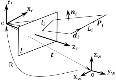
The geometric model of a camera is depicted in Fig. 1. Letc−
xcyczcbe the camera coordinate system with the origin fixed at the focal point, and the axiszccoinciding with the optical axis and pointing to the front of the camera.Idenotes the normalized image plane.o−xwywzwis the object coordinate system.Liis a 3D line in the space andliis its 2D image projection on the image plane. It can be seen that the optical center, the 2D image line li, and the 3D lineLiare on the same plane, which is called the interpretation plane (Dhome et al., 1989). In the object coordinate system,Lican be described asλdi+Pi, wheredi= (dix,d
y i,d
z i)T is the unit direction of the line and,Pi= (xi,yi,zi)Tis an arbitrary point on the line, andλ is a scalar. The 2D image lineliin the camera coordinate system can be expressed as:aix+biy+ci=0. We define a unit vectorni= (ai,bi,ci)T, which representslias (x,y,1)·ni=0. It is clear that ni is the normal vector of the interpretation plane.
The direction vectordiand the pointPican be expressed in the camera coordinate system as Rdiand RPi+t, where the 3×3 rotation matrix R and the translation vectortdescribe the rigid transformation between the object coordinate system and the cam-era coordinate system. Since the two vectors are all in the inter-pretation plane, we have:
nTiRdi=0, (1)
Therefore each line correspondence provides two constraints. E-quations (1) and (2) are the well known fundamental eE-quations of the pose estimation problem from 2D to 3D line correspon-dences (Navab and Faugeras, 1993).
Figure 1: The geometry of the camera model
3 POSE FROM LINE CORRESPONDENCES
We developed a new algorithm of pose estimation from line cor-respondences. Our algorithm is inspired by Lu et al.’s method (Lu et al., 2000) which addresses pose estimation problem from points. In comparison with other algorithms, the iterative method of (Lu et al., 2000) can attain very accurate results in a fast and globally convergent manner. It is regarded as one of the most accurate and efficient pose estimation methods (Moreno-Noguer et al., 2007).
For pose estimation from line features, the existing linear algo-rithms (Ansar and Daniilidis, 2003, Liu et al., 1990) often lacks sufficient accuracy while the iterative algorithms (Phong et al., 1995, Kumar, 1994), which generally uses classical optimization techniques such as Newton and Levenberg-Marquardt method, may not fully exploit the specific structure of the pose estimation problem (Lu et al., 2000), and are usually sensitive to the initial noise or outliers. Our new iterative algorithm is an extension of the algorithm (Lu et al., 2000) to lines, which is named as Line based Orthogonal Iteration algorithm (LOI). Experiments in Sec-t. 4 demonstrate that our method is very efficient and can attain very good performances in terms of both accuracy and robust-ness.
3.1 Object-Space Objective Function
The fundamental equations indicate that each 3D-to-2D line cor-respondence provides 2 constraints. IfN-line correspondences are available, the pose problem becomes the problem of mini-mizing the following objective function (Phong et al., 1995, Lee and Haralick, 1996, Kumar, 1994):
E(R,t) = N
∑
i=1
(nTiRdi)2+ N
∑
i=1
(nTi(RPi+t))2. (3)
Instead of using the objective function of Eq. (3), we present and use an objective metric based on the coplanarity error in the ob-ject space. In fact, just as the collinearity of point correspondence in the way of orthogonal projection (Liu et al., 1990), the copla-narity of a 3D-to-2D line correspondence can be understood in the way that the projection of 3D line in the interpretation plane should be coincide with its self. In the camera coordinate system, the line direction vector is Rdiand its projection in the interpre-tation plane can be obtained by(I−ninTi)Rdiwhere I is a 3×3 identity matrix. Let Ki=I−ninTi, we have:
Rdi=KiRdi. (4)
Similarly, for the point position vector RPi+twe have:
RPi+t=Ki(RPi+t). (5)
From the Eqs. (4) and (5), we have the corresponding vector differences as:
edi = (I−Ki)Rdi, (6)
ePi = (I−Ki)(RPi+t). (7)
We referedi andePi as coplanarity errors. We then achieve the following objective functions:
E1(R) =
N
∑
i=1
∥edi∥2= N
∑
i=1
∥(I−Ki)Rdi∥2, (8)
E2(R,t) = N
∑
i=1
∥ePi∥2=
∑
Ni=1
∥(I−Ki)(RPi+t)∥2. (9)
Compared with Eq. (3), the two objective functions (8) and (9) have clear geometry meaning that the optimal solution of pose should achieve the minimum value of the sum of squares of copla-narity errors (See Fig. 2).
Note that like the line-of-sight projection matrix Videfined in (Li-u et al., 1990), Kiis an interpretation plane projection matrix that, when applied to a object vector, projects the vector orthogonally to the interpretation plane. It owns the following properties:
∥Ki∥ ≥ ∥Kix∥, x∈R3, (10)
KTi =Ki, (11)
K2i =KiKTi =Ki. (12)
Figure 2: Object-Space error of line correspondence
Since our new pose estimation method involves mainly the least-squares estimation, we show a lemma given by the work of (Umeya-ma, 1991) here before proceeding to the details of our method.
Lemma 1: Let A and B bem×nmatrices, and R am×m
rota-tion matrix, and UDVT aSVDof ABT (UUT =VVT =I, D= diag(λi),λ1≥λ2≥ · · · ≥λm≥0). To minimize the objective function
f(R) =∥A−RB∥2, (13)
the optimal rotation matrix R such that
R=USVT. (14)
Whenrank(ABT)
>m−1, S must be chosen as
S=
{
I i f det(ABT)≥0
,
diag(1,1,· · ·,1,−1) else. (15)
Whendet(ABT) =0 (rank(ABT) =m−1), S must be chosen as
S=
{
I i f det(U)det(V) =1,
Algorithm 1:Rotation then Translation
1. GivenN(N≥3) 3D-to-2D line correspondences and initial rotation R0, compute Kifori=1, . . . ,N. Define
B= (d1,d2,· · ·,dN). Setk=0.
2. Perform the following steps:
(a) Compute A= (K1Rkd1,· · ·,KNRkdN).
(b) Compute M=ABTand performSVD: UDVT=M.
(c) Compute Rk+1=USVT, where S is set according to
Eqs. (15) and (16).
(d) Terminate the iteration if convergence is reached; otherwise,k=k+1, go to setp (a).
3. Compute translationtvia (18).
3.2 LOI-1: Rotation then Translation
We propose a pose estimation algorithm which optimizes alterna-tively on the rotation matrix and translation vector.
Lemma 1gives us a solution to the optimal estimate of rotation
matrix R. Let us assume we are givenN3D-to-2D line corre-spondences and we have obtained the projection operator Kifor each correspondence. We define:
A= (K1Rd1,K2Rd2,· · ·,KNRdN),
B= (d1,d2,· · ·,dN).
E1(R)then becomes :
E1(R) =∥A−RB∥2. (17)
It is seen that Eq. (17) bears a close resemblance to Eq. (13). This naturally lets us compute R iteratively as follows: given the estimation rotation matrix Rkatk-th iteration, we compute A(Rk) and seek to minimize∥A(Rk)−RB∥2 to get the next estimate Rk+1 according to the Lemma (1). This step is repeated until
convergence is achieved.
After attaining an estimate of rotation R, the optimal estimate of translationtcan be computed easily by minimizingE2(R,t)of Eq. (9):
t=t(R) = ( N
∑
i=1
(I−Ki))−1 N
∑
i=1
(Ki−I)RPi. (18)
Clearly the matrix(∑Ni=1(I−Ki))must be invertible for Eq. (18) to hold. Since I−Ki=ninTi, we have(∑Ni=1(I−Ki)) =CCT,
where
C=
a1 a2 · · · aN
b1 b2 · · · bN
c1 c2 · · · cN
T
.
Hence ifrank(CCT)≡3, Eq. (18) can be well-defined. In fact, rank(CCT) =rank(C) =3 is always true ifN≥3 and theN in-terpretation planes do not all intersect in one line. In other words, if there are at least three of the 3D lines that do not intersect in one point, the value of translationtcan always be computed by Eq. (18).
We now achieve a two-step pose estimation algorithm(LOI-1): firstly the optimal R∗is iteratively computed, and then the best translationt∗is obtained given the estimated R∗. The algorithm is summarized in Algorithm 1.
3.3 LOI-2: Alternative Optimization
In Algorithm 1, the objective functionE1(R)is minimized firstly
to solve for rotation R. The estimate is then used to minimize the objective functionE2(R,t)to determine the translationt. This
method only uses the information of line direction to compute ro-tation, and doesn’t use the set of constraints effectively. In the framework of solving rotation and translation separately, the s-mall errors in the rotation estimation are amplified into large er-rors in the translation stage (Kumar, 1994). To fully exploit the set of constraints, we can modify Algorithm 1 to optimize alter-natively on the rotation matrix and translation vector.
Assuming we have obtained thek-th estimation of Rk,tkis com-puted viat(Rk). We firstly use the rotation estimation iterative step of Algorithm 1 to estimate a new rotation value R′k+1, and
obtain a new estimate of translationt′k+1viat(R′k+1)from Eq.
(18). Then with (R′k+1,t′k+1), we use the method of (Lu et al.,
2000) to obtain the final (k+1)-th estimation by minimizing the objective functionE2(R,t). The last step is described as follows.
In the algorithm of (Lu et al., 2000), R andtare iteratively opti-mized by minimizing an object space objective function defined for the point correspondences:
E(R,t) = N
∑
i
∥(I−Vi)(RPi+t)∥2, (19)
where Vi is a projection matrix that, when applied to a point, projects the point orthogonally to the line of sight defined by the image point. When Rkand tk are obtained, the next estimate Rk+1is determined by solving the following absolute orientation problem:
Rk+1=arg min
R
N
∑
i=1
∥RPi+t−Viqki∥2, (20)
whereqk
i =RkPi+tk. This absolute orientation problem is then solved bySVDmethod (Horn et al., 1988).
It is seen that the only difference in Eq. (9) compared with Eq. (19) is the use of projection matrix Kiinstead of Vi. Both projec-tion vectors Kiand Vibear the same properties (Sect. 3.1). Hence after we have obtained the estimates (R′k+1,t′k+1), an estimate of
rotation, Rk+1, can be computed by directly using the algorithm
of (Lu et al., 2000) to minimize the objective function (9). The new algorithm is summarized in Algorithm 2.
Obviously if given an initial estimate for both R andt, purely minimizingE2(R,t)by using the the method of (Lu et al., 2000) leads to another algorithm (we denote it as LOI-3). Since the only difference is the definition and use of a projection vector, we will not go further on this algorithm. For more details, the readers are referred to (Lu et al., 2000).
4 EXPERIMENTS
To evaluate our methods, we carried experiments on both syn-thetic and real data.
4.1 Synthetic Data
Algorithm 2:Alternative Optimization
1. GivenN(N≥3) 3D-to-2D line correspondences and initial rotation R0, compute: Kifori=1, . . . ,N,
B= (d1,d2,· · ·,dN). Setk=0.
2. Perform the following steps:
(a) Compute A= (K1Rkd1,· · ·,KNRkdN).
(b) Compute M=ABTand performSVD: UDVT=M.
(c) Compute R′k+1=USVT, where S is set according to Eqs. (15) and (16).
(d) Computet′k+1=t(R′k+1)
(e) Given R′k+1andt′k+1, compute Rk+1using the
algorithm of (Lu et al., 2000).
(f) Computetk+1=t(Rk+1).
(g) Terminate the iteration if convergence is attained; otherwise,k=k+1, go to step (a).
We add Gaussian noise to the projections of points and also con-sider a percentagepoutof outliers, for which a set of 3D lines are randomly selected and replaced by another line generated within the cube[−0.5,0.5]×[−0.5,0.5]×[−0.5,0.5]. For each setting
of the control parameters in every plot, the result is obtained by running 1000 trials and the mean value is recorded. To facilitate the description, we denote the Algorithm 1∼3 as LOI-1, LOI-2 and LOI-3 separately.
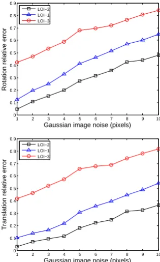
In Fig. 3, we plot the rotation and translation relative errors pro-duced by the three algorithms as a function of Gaussian noise with its standard deviation varies from 1 to 10 pixels. The num-ber of sampling points that are used for creating the 2D lines is set as 100. The line number is fixed to be 8 and the percentage of outlierspout=0. The plots show that “LOI-2” is consistently more accurate than the other two algorithms.
1 2 3 4 5 6 7 8 9 10 0
0.1 0.2 0.3 0.4 0.5 0.6 0.7 0.8 0.9
Gaussian image noise (pixels)
Rotation relative error
LOI−2 LOI−1 LOI−3
1 2 3 4 5 6 7 8 9 10 0
0.1 0.2 0.3 0.4 0.5 0.6 0.7 0.8 0.9
Gaussian image noise (pixels)
Translation relative error
LOI−2 LOI−1 LOI−3
Figure 3: Relative rotation and translation error as a function of image noise when the number of lines is fixed to be 8.
Fig. 4 plots the errors as the function of the number of 3D object
lines when the image noise is fixed (σ=3 pixels). We compare the performances of our algorithms with the OI method (Lu et al., 2000), for which the corresponding 2Nendpoints of the 3D lines are used. It can be seen that all these algorithms can achieve higher accuracy when the number of feature correspondence in-creases. LOI-2 and OI algorithms show more accurate and stable performances.
5 10 15 20
0 0.1 0.2 0.3 0.4 0.5 0.6 0.7 0.8 0.9 1
Number of 3D object lines
Rotation relative error
LOI−2 LOI−1 LOI−3 OI
5 10 15 20
0 0.1 0.2 0.3 0.4 0.5 0.6 0.7 0.8 0.9 1
Number of 3D object lines
Translation relative error
LOI−2 LOI−1 LOI−3 OI
Figure 4: Relative rotation and translation error as a function of the number of object lines when the standard deviation of image noise is fixed to be 3 pixels.
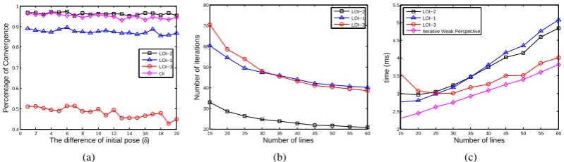
In Fig. 5(a), we give the percentage of convergence when the initial poses are generated from a multinormal distribution with mean as the true pose and the diagonal covarianceδ Σ0, where the standard deviation element ofΣ0is about 1.5 degree for the rotation angles, 0.2 for thexandycomponents of the translation t, and 0.5 for thezcomponent. δvaries from 1 to 20. The plot indicates that LOI-2 shows very robust performance and slightly outperforms the OI algorithm which is proved to be global con-vergent. In contrast, the LOI-3 algorithm produces very poor per-formance. We conclude that, without exploiting the direction in-formation of the lines, LOI-3 is very sensitive to the image noise as well as to the initial pose. Fig. 5(b) plots the number of it-erations as the function of the number of object lines. With the increase of the line number, the number of iterations needed de-creases. Since in LOI-2 there are two updates of rotation, the computation time taken by 1 iteration in LOI-2 is about double of that in LOI-1 and LOI-3. This can be seen from Fig. 5(c), which gives the computation times. The LOI-1 and LOI-2 use almost the same running times. LOI-3 is faster with the increas-ing of the number of lines. We compare our methods with the iterative weak perspective (IWP) method (Christy and Horaud, 1999), which estimates a pose with a weak perspective camera model and improves the estimation iteratively by solving an ap-proximate system of linear equations. Our orthogonal iteration methods are very efficient and comparable to the IWP method.
4.2 Real Data
0 2 4 6 8 10 12 14 16 18 20 0.4
0.5 0.6 0.7 0.8 0.9 1
The difference of initial pose (δ)
Percentage of Convergence
LOI−2 LOI−1 LOI−3 OI
(a)
15 20 25 30 35 40 45 50 55 60 20
30 40 50 60 70 80
Number of lines
Number of iterations
LOI−2 LOI−1 LOI−3
(b)
15 20 25 30 35 40 45 50 55 60 2
2.5 3 3.5 4 4.5 5 5.5
Number of lines
time (ms)
LOI−2 LOI−1 LOI−3 Iterative Weak Perspective
(c)
Figure 5: (a) the number of iterations and (b) the running times as a function of the number of lines. (c) the percentage of convergence when initial poses are generated from a multinormal distribution.
The tracking is performed on an image sequence recorded from a moving calibrated camera pointing towards the scene as shown in Fig. 6. We implement a simple line tracker in a typical frame-work where a local search along the normal direction of a model edge line is performed for gradient maxima for a set of sampled points in the line (Wuest et al., 2005). The strong maxima are taken as the 2D feature points whose corresponding 3D sampled points are in the object line. At run time, the tracker generates a set of 3D-to-2D line correspondences among which outliers or erroneous ones exist. Robust pose estimation method that well re-sists outliers is evaluable for robust tracking. We use our method, LOI-2 specifically, for the tracking. Fig. 6 shows four frames of the tracked sequence. Our method consistantly tracks the whole sequence.
5 CONCLUSIONS AND FUTURE WORK
Robust pose estimation is necessary for refining the pose. We p-resented efficient and robust iterative pose estimation algorithms for line features. Our method introduces coplanarity errors and formulates objective function in the object space by employing orthogonal projections. In the same framework, three pose esti-mation algorithms are given and their performances are evaluat-ed. Compared with other pose estimation algorithm for lines, one of the proposed methods-LOI-2 algorithm is extremely robust, accurate, and also converges fast.
For future work, we are interested in using our methods for real applications, for example, robot navigation. By making use of more other information like the appearance of object, the search of pose from unknown line correspondences may speed up. We are also interested in implementing our simultaneous pose and correspondence method on GPU, for real-time virtual reality ap-plications.
REFERENCES
Ansar, A. and Daniilidis, K., 2003. Linear pose estimation from points or lines. IEEE transactions on pattern analysis and ma-chine intelligence.
Chen, H. H., 1991. Pose determination from line-to-plane cor-respondences: Existence condition and closed-form solutions. IEEE transactions on pattern analysis and machine intelligence.
Christy, S. and Horaud, R., 1999. Iterative pose computation from line correspondences. Computer vision and image understanding.
Dhome, M., Richetin, M., thierry Lapreste, J. and Rives, G., 1989. Determination of the attitude of 3-D objects from a sin-gle perspective view. IEEE transactions on pattern analysis and machine intelligence.
Haralick, R. M., Joo, H., Lee, C.-N., Zhuang, X., VAIDYA, V. G. and Kim, M. B., 1989. Pose estimation from corresponding point data. International Journal of Computer Vision.
Horaud, R., dornaika, F., Lamiroy, B. and christy, S., 1997. Ob-ject pose: the link between weak perspective, paraperspective, and full perspective. International Journal of Computer Vision 22(2), pp. 173–189.
Horn, B. K. P., Hilden, H. and Negahdaripour, S., 1988. Closed-form solution of absolute orientation using orthonormal matrices. Journal of the Optical Society America 5(7), pp. 1127–1135.
Kumar, P., 1994. Robust methods for estimating pose and a sen-sitivity analysis. Image understanding 60(3), pp. 313–342.
Lee, C.-N. and Haralick, R. M., 1996. Statistical estimation for exterior orientation from line-to-line correspondences. Image and vision computing 14, pp. 379–388.
Liu, Y., Huang, T. S. and Faugeras, L. D., 1990. Determination of camera location from 2-D to 3-D line and point correspondences. IEEE transactions on pattern analysis and machine intelligence.
Liu, Y., Huang, T. S. and Faugeras, O. D., 1988. A linear algo-rithm for motion estimation using straight line correspondences. Computer Vision Graphics Image Processing.
Lu, C.-P., Hager, G. D. and Mjolsness, E., 2000. Fast and globally convergent pose estimation from video images. IEEE transaction-s on pattern analytransaction-sitransaction-s and machine intelligence.
Moreno-Noguer, F., Lepetit, V. and Fua, P., 2007. Accurate non-iterative O(n) solution to the PnP problem. In: IEEE Conference on Computer Vision and Pattern Recognition.
Navab, N. and Faugeras, O., 1993. Monocular pose determination from lines: Critical sets and maximum number of solutions. In: IEEE Conference on Computer Vision and Pattern Recognition.
Phong, T. Q., Horaud, R., Yassine, A. and Tao, P. D., 1995. Ob-ject pose from 2d to 3d point and line correspondences. Interna-tional Journal of Computer Vision 15(3), pp. 225–243.
Quan, L. and Lan, Z., 1999. Linear N-point camera pose de-termination. IEEE transactions on pattern analysis and machine intelligence.
Umeyama, S., 1991. Least-squares estimation of transformatio parameters between two point patterns. IEEE transactions on pat-tern analysis and machine intelligence.
(a) frame #1 (b) frame #52
(c) frame #86 (d) frame #135