www.elsevier.comrlocaterapplanim
Least-effort pathways?: a GIS analysis of livestock
trails in rugged terrain
D. Ganskopp
a,), R. Cruz
b, D.E. Johnson
ca
USDA-Agricultural Research SerÕice and EOARC1, HC-71 4.51 Highway 205, Burns, OR 97720, USA
b
Calle Cunduacan No. 110, Fraccionamiento Plaza Villahermosa, Villahermosa, Tabasco C.P. 86179, Mexico
c
Department of Rangeland Resources, Oregon State UniÕersity, CorÕallis, OR 97731, USA
Accepted 17 January 2000
Abstract
Livestock trails frequently evolve in pastures when plant growth or establishment cannot keep pace with vegetation disturbance. In some instances, man-made trails are established in rangeland settings to encourage uniform use of forages or facilitate livestock passage through dense vegetation or across rugged terrain. A long-term assumption has been that livestock establish pathways of least resistance between frequented areas of their pastures, but this hypothesis has never been tested. We mapped cattle trails in three 800qha pastures with global positioning
Ž .
units. A geographic information system GIS helped quantify characteristics of trails and the landscape and was used to plot least-effort pathways between water sources and distant points on selected trails in the pastures. Characteristics of the cattle trails and least-effort pathways were compared to test the hypothesis that cattle develop least-effort routes of travel in rugged terrain. The mean slope of the three pastures was 13.5%, and the average slope of the topography traversed by the cattle trails was 8%. The slope of the trails was reduced to 5.2% by selection of cross-slope routes. When we compared the characteristics of 10 selected cattle trails and
Ž .
least-effort pathways generated by our GIS, the cattle trails were 11% shorter Ps0.046 than the least-effort pathways, and the topography traversed by cattle had a gradient about 1% less than the
Ž . Ž . Ž .
least-effort pathways Ps0.02 . The slope of the selected trails 5.5% and pathways 5.6%
Ž .
were similar Ps0.74 , however. Analyses of values extracted from cost surfaces indicated that,
)Corresponding author. USDA-Agricultural Research Service, HC-71 4.51 Highway 205, Burns, OR 97720, USA. Tel.:q1-541-573-2064; fax:q1-541-573-3042.
Ž .
E-mail address: [email protected] D. Ganskopp .
1
Eastern Oregon Agricultural Research Center, Including the Burns and Union Stations, is jointly operated by the Oregon Agricultural Experiment Station of Oregon State University and the USDA-Agricultural Research Service.
0168-1591r00r$ - see front matterq2000 Elsevier Science B.V. All rights reserved.
Ž .
on the average, 183 units of effort were needed to traverse the trails and 170 units of effort
Ž .
expended to traverse the least-effort pathways Ps0.07 . These data support the hypothesis that cattle establish least-effort routes between distant points in rugged terrain and suggest that GIS software may be useful in designing systems of livestock trails in extensive settings. q2000 Elsevier Science B.V. All rights reserved.
Keywords: Cattle feeding and nutrition; Rangeland; Optimum foraging; Global positioning system; GPS;
Geographic information system; Foraging; Grazing behavior; Efficiency
1. Introduction
One consequence of repetitive travel by livestock on rangelands is the formation of
Ž
trails. Since cattle innately move among locations in single file Weaver and Tomanek,
.
1951; Arnold and Dudzinski, 1978 , trails frequently evolve in pastures when plant
Ž
growth or establishment cannot keep pace with vegetation disturbance Walker and
.
Heitschmidt, 1986 . In rangeland pastures, trails typically connect necessary but limited resources like water, shade, forage, or mineral sources. In some instances, man-made trails have been used to encourage uniform use of forages or facilitate livestock passage
Ž .
through dense vegetation or rugged terrain Vallentine, 1974 .
It has long been assumed that livestock establish pathways of least resistance between
Ž
frequented portions of their pastures Weaver and Tomanek, 1951; Arnold and
Dudzin-.
ski, 1978 , but this hypothesis has never been tested. Such a hypothesis might be
Ž .
considered a component of MacArthur and Pianka’s 1966 optimum foraging theory, whereby animals are expected to minimize energy expenditures while maximizing energy gains in their daily endeavors.
Foraging activities and questions of energy optimization are difficult to quantify in
Ž .
practice, but recent advances in Geographic Information Systems GIS and Global
Ž .
Positioning Systems GPS have greatly simplified examination of many spatially related phenomena. As part of a long-term effort to model the spatial dynamics of livestock distribution, the objectives of this research were to quantify the extent and characteristics of cattle trails in three large pastures and indirectly test the hypotheses
Ž .
that cattle 1 reduce energy expenditures by traversing the more gentle topography in
Ž .
their pastures, 2 they further reduce energy expenditures by selecting cross-slope
Ž .
routes, and 3 they use least-effort pathways when traveling between distant points. These were accomplished by mapping livestock trails with a GPS unit and quantifying their characteristics and those of the associated landscape with GIS software.
2. Methods
2.1. Study area
Ž X Research was conducted at the Northern Great Basin Experimental Range 119843 W,
X .
43829 N; elevation 1425 m about 72 km west–southwest of Burns, OR. Mean annual
precipitation is 28.9 cm with about 60% of the annual accumulation being snow. Mean annual temperature is 7.68C with recorded extremes ofy298C and 428C. Vegetation is
Ž .
Ž .
A shrub layer is dominated by low sagebrush Artemisia arbuscula Nutt. , Wyoming
Ž .
big sagebrush Artemisia tridentata subsp. wyomingensis Beetle or mountain big
Ž Ž . .
sagebrush Ar. tridentata subsp. Õaseyana Rydb. Beetle . The herbaceous dominants
Ž Ž . .
include bluebunch wheatgrass Agropyron spicatum Pursh Scribn. and Smith , Idaho
Ž . Ž .
fescue Festuca idahoensis Elmer , or Sandberg’s bluegrass Poa sandbergii Vasey .
Ž .
The three largest pastures 825–859 ha on the experimental range were used in this study. In 1996 and 1997, each pasture was stocked with 40 Hereford=Angus cowrcalf pairs from approximately 20 May to 20 September. With the exception of two to three replacement animals per pasture, the same cows grazed each pasture each year. Water and salt were furnished from a roughly centralized source in each of the pastures with no shifts in location between years.
In years prior to the study, all three pastures had a sporadic history of seasonal use by up to 200 cowrcalf pairs. In those instances, pastures were stocked for much shorter intervals, and water and salt were simultaneously available from three to five different sources in each pasture. All of the cattle used in this study were born on the station, and at one time or another had experience with all of the station’s properties.
( ) 2.2. Digital eleÕation model DEM
A DEM, derived from USGS 7.5 min topographic maps, was available for the entire Experimental Range, and was used in conjunction with GIS software to characterize several attributes of our pastures and cattle trails. Unlike conventional topographic maps where elevations are associated with individual lines on the image, every x and y coordinate or pixel on a DEM is assigned an elevation through an interpolation and rasterization process. A pixel is the smallest unit of the map for which information is available, and its area ultimately defines the resolution of the map. On our images, a pixel represented a surface area of 26.73 m2 or a square 5.17 m to a side. Thus, a map
encompassing 850 ha would contain 317,995 pixels. Fig. 1 DEM illustrates the conceptual relationships of data in a rasterized DEM for a synthesized 25 m2area. When
a DEM is viewed with GIS software, each elevation may be depicted by a specific color, and the precise coordinates and elevation of any location on the image can be displayed or extracted for other analyses. After our DEM was complete, we again used the GIS software to generate other maps of the same pastures. These included maps depicting
Ž . Ž . Ž . Ž .
degree of slope DS , percent slope PS , and aspect Aspect of the topography Fig. 1 . In aspect maps, the value associated with each pixel is an azimuth or compass heading indicating the direction one must travel to move downhill most rapidly. An east-facing slope for example would have an aspect of 908, while a west-facing slope would have an
aspect of 2708. Slopes facing north have an aspect of 3608, and level ground has an
aspect of zero because there is no direction that facilitates downhill travel.
2.3. GPS mapping
In July and August of 1997, we surveyed the cattle trails in all three pastures using a Trimble GeoExplorer2 GPS unit. The unit was configured to integrate its position every
2
Fig. 1. A rendition of the spatial arrangement of data in a geographic information system for a DEM of a
Ž 2 .
synthesized 5=5 m landscape 1 m per pixel . Elevations on the DEM range from a low of 1.875 m at the
Ž .
corners to a high of 2.05 m in the center. Two digital slope models, expressed in both degrees DS and
Ž .
percent slope PS , illustrate the gradient of the landscape. The ASPECT image directs one toward the azimuth
Ž .
or compass heading yielding the most rapid rate of descent. After identifying a starting point source , a
Ž .
geographic information system can integrate an aspect image and a friction surface DS degrees to derive a
Ž .
Ž .
5 s and output coordinates to a file using the Universal Transverse Mercator UTM projection. At our rates of walking, it determined a position and saved it to memory every 6 to 7 m.
Coordinates generated by civilian GPS units are generally accurate to within"100 m of the unit’s true position. Inaccuracies are primarily intentional errors introduced by the United States Department of Defense. Much of the intentional error, however, can be removed using differential correction, a process which uses simultaneously collected data from a nearby base station or a stationary GPS unit placed at an accurately
Ž
surveyed position. We obtained base station files from a cooperatively managed US
. Ž
Forest ServicerBureau of Land Management unit in Burns, OR http:rr
.
www.fs.fed.usrdatabasergpsrburns.htm .
After differential correction, coordinates are typically within 1.3 m of their true position. Our GPS unit’s memory and battery capacities allowed continuous operation and data storage for up to 14 h. Mapping of the cattle trails initially began at a pasture’s water source. The beginning of each trail was marked with a flag, and its length traversed until no evidence of repeated livestock use was evident. The endpoint was flagged, and we returned to any previously noted forks in the trail and repeated the process. Abandoned trails that had been used when pastures were more heavily stocked and densely watered were not surveyed. In most instances, those routes led to alternative watering sites that were abandoned in 1995.
Near areas where cattle tended to concentrate, trails occasionally exhibited a braided configuration. In these instances, smaller trails branched off from main thoroughfares
Ž .
only to rejoin the main route after a short 10–50 m distance. These braids probably allow simultaneous passage of animals moving in opposing directions. Obvious braids were not included in our sampling, so our data do not furnish a complete inventory of trail-affected landscape in our pastures.
The differentially corrected coordinates were entered into our GIS system, overlaid on the DEM of the appropriate pasture, and the elevation extracted for each data point. The resulting file contained x and y coordinates and an elevation for each coordinate defining the trail. Typical GPS units can indeed estimate elevation, but error is much smaller when elevations are extracted from a DEM.
2.4. Distance and slope measurements
Custom software was developed to cumulatively tally the distance and percent slope
Ž .
between successive coordinates along each trail. The distance D between successive
2 2
(
points is equal to
Ž
x2yx1.
qŽ
y2yy1.
where x , y and x , y are the respective1 1 2 2 Ž .rectangular coordinates of points 1 and 2. The percent slope S between two successive coordinates
<e2ye1<
s
Ž
100.
D
topography that was traversed by a trail, because animals do not always move straight up or down a hill. To quantify the slope of the topography traversed, we superimposed
Ž .
the coordinates defining the trails on the percent slope PS image and extracted the slope values of the underlying pixels.
2.5. Cost surfaces
A feature common to many GIS systems is an ability to derive least-effort or least-cost pathways across a landscape. Typical uses of these applications include tasks like highway or pipeline design. We used this feature to test our hypothesis that cattle establish least-effort routes between the only water source in a pasture and three to four distant points or targets along different trails in each pasture. The first step in this process required development of a new GIS image of each pasture called a cost surface, which was an integration of two separate images. The first image used was a friction surface where each pixel contained a measure or value defining the resistance or difficulty encountered when traversing the landscape. In this instance, we used DS images as friction surfaces, where the value associated with each pixel was the DS for the underlying topography. Because the algorithm used by our GIS system assumed that one must overcome at least one unit of friction when traversing level ground, a value of 1 was added to each pixel in the DS image. Thus, values of individual pixels in our friction surfaces ranged from 1 on level terrain to 91 where vertical cliffs occurred.
In the simplest applications, cost surfaces may be derived directly from a friction surface. In those instances, one first establishes a ‘‘source’’ or starting position on the friction surface. The software then generates a cost surface by simply summing the friction values that it must traverse to reach each location or pixel on the landscape and the totals are assigned to each of the destination pixels on the newly generated cost surface. On the cost surface, the lowest value occurs at the source or starting position, and the highest values are typically found at the most extreme distances. An example where this model would suffice might involve moving through various accumulations of snow deposited on level terrain. In that instance, the friction surface would simply depict various depths of snow across the landscape, and individual pixels on the cost surface would reflect the sum of the depths one traversed to reach each point.
When traveling across rugged terrain, however, gravity and DS have directional attributes that may help or hinder one’s movement. As one moves downslope, gravity essentially applies additional force to one’s back that facilitates motion. Conversely, as one moves upslope, gravity becomes an impediment, and one must overcome additional friction to make progress.
To incorporate this directional component into the cost surface, the GIS software
Ž .
integrated the DS friction surface , and aspect images of each pasture. Again, each pixel
Ž .
in an aspect image is an azimuth compass heading directing one towards the steepest route of descent. If one travels along the azimuth, the force of gravity is maximized and
Ž .
movement is facilitated force . Conversely, travel in an uphill direction 1808away from
the azimuth is impeded by the additional friction effect of gravity. Travel in a direction
Ž .
908either side of the azimuth i.e. parallel to a contour is equated with movement on
Where travel was not parallel to the azimuth, the amount of friction or force was
Ž f. 2
adjusted by a cosine function i.e. effective frictionsstated friction where fscosa
anda is the difference angle between the angle of travel selected and the direction from .
which friction or force was maximum . As the cost surface was assembled, successive
Ž .
friction accumulations uphill movements were incremented by values greater than 1,
Ž .
while increments of force downhill travel incurred additions that were reciprocals of the effective friction. As an example of the calculations, let us assume a hillside has a
Ž .
slope of 98thereby yielding a stated friction of 10 i.e. 9q1 . The hill has an aspect of
Ž .
458 faces northeast and one’s direction of travel is an upslope heading of 2658. The
difference angle between the aspect and ones heading is 2208, fs0.5868, and the
effective friction or cost for traversing a pixel is 100.5868 or 3.862. If one reversed
direction and moved downslope on a heading of 858, the difference angle becomes 408,
Ž .
and 0.259 units of force the reciprocal of 3.862 are accumulated when traversing the same pixel.
After a cost surface was assembled for a pasture, we arbitrarily selected coordinates for three to four target locations in each pasture. These target coordinates were on the cattle trails and located as far as possible from the water source in each pasture. The GIS
Ž .
software then derived least-cost pathways between the source water tank and target coordinates. This is accomplished by conceptually placing one’s self at a target location on the cost surface, examining each of the surrounding pixels for the lowest possible
Ž .
value, and stepping to that pixel Fig. 1 — Cost surface . The process continues until
Ž .
the system encounters the lowest value on the cost surface zero , which was the location of the water source. Each cattle trail and its associated least-cost pathway was superimposed on its respective cost surface, and the mean cost of traversing each route determined by extracting the values of the underlying pixels. Pathway length, slope of the topography traversed by the pathway, and slope of the least-cost pathways were determined with the same methods used previously for the trails. Three trailrpathway comparisons were generated from both Pastures 1 and 2, and 4 comparisons were generated in Pasture 7, for a total of 10 paired observations.
2.6. Hypothesis testing
Four criteria were used to test our hypothesis that cattle use least-effort pathways
Ž .
when traveling between distant points. Comparisons included measures of: 1 length
Ž . Ž .m ; 2 slope of the topography traversed % ; 3 slope of the selected routes % ; andŽ . Ž . Ž . Ž .4 an index of travel costs incurred when traversing cattle trails and least-effort
pathways. Paired trailrpathway routes were considered an experimental unit, and paired
Ž .
t tests 9 df were used to evaluate disparities between the two routes. If no significant
trailrpathway disparities occurred among the four criteria, we would accept our least-effort hypothesis. Conversely, if cattle trails were longer than pathways, traversed steeper grades than pathways, or incurred higher travel costs than pathways, we would reject our least-effort hypothesis.
To test our hypotheses that cattle reduce travel efforts by selecting more gentle topography and further reduce travel effort by selecting cross-slope routes, we again
Ž .
pastures, the mean slopes the areas traversed by trails, and the slope of the cattle trails. In these analyses, a pasture was considered an experimental unit. Statistical significance in all analyses was accepted at PF0.05.
3. Results
3.1. Trail characteristics
A total of 50 km of trails were mapped in the three pastures with 7578 coordinates
Ž .
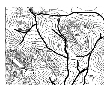
available to quantify characteristics of the trails Table 1 . Over 300,000 data points were available to describe landscape characteristics in each of the pastures. The general topography, location of the water source, and distribution of cattle trails for one of the three pastures is illustrated by Fig. 2. Trails extended to the lowest elevations in two of
Ž .
the three pastures Pastures 1 and 2 , but were from 18 to 135 m short of reaching the
Ž .
highest elevations in all instances Table 1 . Watering facilities were within 13 to 21 m of the mean elevation of each pasture.
Total length of trails in each pasture ranged from 12.9 to 19.6 km, and mean density
2 Ž .
of trails was 2 kmrkm of pasture Table 2 . Slope of the topography in our pastures
Ž . Ž .
averaged 13.5%, and cattle trails traversed significantly P-0.01 lesser grades 8% than one would expect from examination of pasture means. Average slope of the trails
Ž .
was 5.2%, which was significantly P-0.01 less than the mean slope of the pastures or of the topography traversed by the trails.
3.2. Trailrpathway comparisons
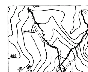
Examination of cattle trails and least-effort pathways targeting the same coordinates suggested that roughly similar routes were selected, but trails and pathways were not
Ž . Ž .
identical tracings Fig. 3; Table 3 . On average, cattle trails were 11% shorter Ps0.046
Table 1
Area, topographic characteristics, and number of data points describing the landscape, water sources, and cattle trails in three rangeland pastures on the Northern Great Basin Experimental Range near Burns, OR in 1997 Characteristic Pasture
1 2 7
Landscape Trails Landscape Trails Landscape Trails
Ž .
Area ha 825 – 853 – 859 –
Ž .
Lowest elevation m 1395 1395 1400 1400 1414 1419
Ž .
Highest elevation m 1608 1550 1670 1535 1579 1561
Ž .
Mean elevation m 1483 1465 1483 1472 1488 1469
Ž .
Water elevation m 1496 – 1504 – 1469 –
Ž .
Ž . Ž .
Fig. 2. Topography 6.1 m contour lines and extent of cattle trails heavy dark lines in Pasture 1 on the Northern Great Basin Experimental Range near Burns, OR in 1997.
than least-effort pathways, and the topography traversed by cattle had a slope about 1%
Ž . Ž .
less than least-effort pathways Ps0.02 . The slope of the trails 5.5% and pathways
Ž5.6% were similar P. Ž s0.74 , however, and analyses of the values extracted from cost.
Ž . Ž .
surfaces Fig. 3 suggested the effort to traverse the trails xs183 and pathways
Žxs170 was also similar P. Ž s0.07 ..
Table 2
Total length of cattle trails, densityrkm2of trails, mean slope of pastures, mean slope of topography traversed by trails, and slope of cattle trails in three rangeland pastures on the Northern Great Basin Experimental Range near Burns, OR in 1997
Characteristic Pasture 1 Pasture 2 Pasture 7 Mean
Ž .
Total length of trails km 19.6 17.6 12.9 16.7
2
Ž .
Density of trails kmrkm 2.4 2.1 1.5 2.0
a
Ž .
Mean slope of entire pasture % 15.2 12.5 12.7 13.5a
Ž .
Mean slope of areas traversed by trails % 8.7 7.1 8.0 8.0b
Ž .
Mean slope of trails % 5.4 4.5 5.2 5.2c
a Ž .
Ž . Ž .
Fig. 3. Cattle trails open parallel lines and least-effort pathways heavy dark lines from the only water source to three selected coordinates in Pasture 1 on the Northern Great Basin Experimental Range near Burns, OR in 1997. Contour lines represent increments of 50 units of effort and were derived from the cost surface for Pasture 1. Values on the cost surface range from zero at the water source, where the routes converge, to a maximum of 461 near the northwest corner of the pasture.
Table 3
Length, slope characteristics, and travel costs of cattle trails and least-effort pathways to selected points in three pastures on the Northern Great Basin Experimental Range near Burns, OR in 1997
Ža, b Paired trail. rpathway means sharing a common letter are not significantly different PŽ )0.05 ..
Ž . Ž .
Pasture Routea Length Mean % slope Mean % Mean travel
Ž .m traversed slope cost
Trail Pathway Trail Pathway Trail Pathway Trail Pathway
1 1 2808 3066 9.6 11.0 5.5 6.8 174 161
2 2820 2977 7.5 9.6 4.7 6.4 214 187
3 2556 2556 8.1 10.2 7.1 7.1 165 172
2 1 2181 2322 3.0 2.3 2.0 1.8 148 154
2 2026 2212 6.4 6.5 3.8 4.0 177 167
3 2280 2564 10.7 11.0 7.8 7.5 182 160
3 1 1998 2077 5.7 7.2 4.0 4.2 164 160
2 1864 3026 13.7 14.4 8.2 6.1 315 260
3 2154 2265 5.0 5.8 3.2 3.8 144 141
4 932 991 11.2 11.5 8.6 7.3 143 142
4. Discussion and conclusions
While the most extreme slopes in our pastures were grades of 167%, 95% of our pasture surface occurred where slopes were less than 38%. Cattle typically use less
Ž .
resources in areas where grades approach 30% Van Vuren, 1982 . They prefer foraging on slopes in the 0–9% category, are indifferent to slopes between 10% and 19%, and
Ž .
avoid grades exceeding 20% Ganskopp and Vavra, 1987 . While energy costs of movement through rugged terrain have not been documented in cattle, Parker et al.
Ž1984 suggest the costs of lifting a kilogram one vertical meter is 5.9 kcal for wild and. Ž .
domestic ungulates regardless of body weight or species. Yousef et al. 1972 , however, monitored oxygen consumption of burros on level ground and on grades up to 17% and noted that energy costs did not increase linearly with slope. An increase in grade from 10% to 17% created a much higher rate of oxygen consumption than predicted with a shift from a 2% to 10% slope. Our algorithm for estimating travel cost was curvilinear in
Ž .
nature, and examination of figures supplied by Yousef et al. 1972 suggests that this might be an appropriate form for a model. Nevertheless, our cost surfaces may not provide an accurate reflection of the energy expenditures incurred by cattle, and more research is needed to accurately quantify their energy requirements as they ascend and descend slopes of varying difficulty.
Despite this shortcoming, our procedures still provided vigorous tests of the various hypotheses. Our hypothesis that cattle reduce their energy expenditures by traversing less rugged terrain was supported by the disparity between the mean slope of the
Ž . Ž .
pastures 13.5% and the mean slope of the topography traversed by cattle trails 8% . The slope of the trails averaged 5.2% again supporting our hypothesis that energy expenditures were further reduced by the selection of cross-slope routes. Examples of
Ž .
this can be seen near the four corners of Pasture 1 Fig. 2 where trails appear to be oriented nearly parallel with the contour lines.
If we accept the assumption that GIS software is capable of deriving least-cost pathways, then our hypothesis that cattle used least-effort routes was also well sup-ported. On the average, cattle selected routes that were 243 m shorter than the GIS
Ž .
pathways, the slopes traversed by the cattle occurred on about 1% less grade P-0.05 than GIS pathways, and the slopes and associated travel costs of the trails and pathways were equivalent.
We suspect that a portion of the difference in length between the trails and pathways was a product of the algorithms used in derivation of the pathways. Close scrutiny of the
Ž .
paired routes Fig. 3 revealed that pathways exhibited a more jagged and less direct line of travel than the cattle trails. Possibly, the cattle were more efficient at averaging over longer reaches of topography and slightly more goal oriented than the computer that only looked one step ahead as it selected a least-effort route. Development of GIS algorithms that examine a larger spatial window might partially eliminate this disparity. Given that the cattle trails exceeded or equaled the computer’s capacities, however, we accepted the hypothesis that cattle follow paths of least resistance.
to cattle before extensive resources are committed or extended reaches of vegetation are disturbed.
Additionally, we noted two circumstances in our pastures where cattle apparently established one-way systems of trails. Supporting evidence included observation of cattle movements and the orientation of their tracks on the trails. In both instances, cattle ranged out from water and selected an alternative and more circuitous route for their return trip. We briefly examined this observation by generating new cost surfaces of the two pastures where these observations occurred. The distant destination points accessed by these trails were reclassified as sources, and the water tanks were reclassified as targets. The derived pathways closely paralleled routes used by the cattle to return to water.
In both of these cases, the one-way trails left the water source and descended steep
Ž20–40% slopes to a lower plain. The cattle would subsequently return to water via. Ž .
longer but less steeply inclined routes. When descending a steep grade 17% , burros use
Ž .
only about 1r3 of the oxygen required to climb the same path Yousef et al., 1972 , so selection of longer but less steeply inclined return routes may be a cost-effective means of travel is rugged environments. We need to document more instances of this behavior, however, before these observations can be substantiated. Should one elect to use a GIS system to design livestock trails, we suggest that pathways for travel be explored in both directions, especially when cattle are expected to traverse long reaches of steep slopes exceeding a 20% grade. If substantially different pathways are generated from these analyses, then managers may need to develop both routes before cattle will effectively use resources in the desired locale.
References
Arnold, G.W., Dudzinski, M.L., 1978. Developments in Animal and Veterinary Sciences: 2. Ethology of Free-ranging Domestic Animals. Elsevier, New York.
Ganskopp, D., Vavra, M., 1987. Slope use by cattle, feral horses, deer, and bighorn sheep. Northwest Sci. 61, 74–81.
MacArthur, R.H., Pianka, E.R., 1966. On optimal use of a patchy environment. Am. Nat. 100, 603–609. Parker, K.L., Robbins, C.T., Hanley, T.A., 1984. Energy expenditures for locomotion by mule deer and elk. J.
Wildl. Manage. 48, 474–488.
Vallentine, J.F., 1974. Range Development and Improvements. Brigham Young Univ. Press, Provo, UT, p. 516.
Van Vuren, D., 1982. Comparative ecology of bison and cattle in the Henry Mountains, Utah. In: Peek, J.M.,
Ž .
Dalke, P.D. Eds. , Proc. Wildlife–livestock Relationships: Symp.. Dept. of Wildl. Res., College of Forestry, Wildlife and Range Sciences, University of Idaho, Moscow, pp. 449–457.
Walker, J.W., Heitschmidt, R.K., 1986. Effect of various grazing systems on type and density of cattle trails. J. Range Manage. 39, 428–431.
Weaver, J.E., Tomanek, G.W., 1951. Ecological studies in a Midwestern range: the vegetation and effects of cattle on its composition and distribution. Nebr. Conserv. Bull. 31.
Yousef, M.K., Dill, D.B., Freeland, D.V., 1972. Energetic cost of grade walking in man and burros, Equus