Minimizing stochastic complexity using local search and
GLA with applications to classification of bacteria
P. Fra¨nti
c, H.G. Gyllenberg
e, M. Gyllenberg
a,b, J. Kivija¨rvi
a, T. Koski
a,d,
T. Lund
a,*, O. Nevalainen
a,baDepartment of Mathematical Sciences,Uni6ersity of Turku,FIN-20014 Turku, Finland bTurku Center for Computer Science (TUCS),Uni6ersity of Turku,FIN-20014 Turku, Finland cDepartment of Computer Science,Uni6ersity of Joensuu,P.O. Box111,FIN-80101 Joensuu, Finland
dDepartment of Mathematics,Royal Institute of Technology,10044 Stockholm, Sweden eInstitute of Biotechnology,Uni6ersity of Helsinki,00014 Helsinki, Finland
Received 2 September 1999; received in revised form 13 April 2000; accepted 17 April 2000
Abstract
In this paper, we compare the performance of two iterative clustering methods when applied to an extensive data set describing strains of the bacterial family Enterobacteriaceae. In both methods, the classification (i.e. the number of classes and the partitioning) is determined by minimizing stochastic complexity. The first method performs the minimization by repeated application of the generalized Lloyd algorithm (GLA). The second method uses an optimization technique known as local search (LS). The method modifies the current solution by making global changes to the class structure and it, then, performs local fine-tuning to find a local optimum. It is observed that if we fix the number of classes, the LS finds a classification with a lower stochastic complexity value than GLA. In addition, the variance of the solutions is much smaller for the LS due to its more systematic method of searching. Overall, the two algorithms produce similar classifications but they merge certain natural classes with microbiological relevance in different ways. © 2000 Elsevier Science Ireland Ltd. All rights reserved.
Keywords:Classification; Stochastic complexity; GLA; Local search; Numerical taxonomy
www.elsevier.com/locate/biosystems
1. Introduction
Minimization of stochastic complexity (SC) (Rissanen, 1989) has proven to be an efficient method in numerical taxonomy, that is, in the classification and identification of bacteria based on phenetic features (Gyllenberg et al., 1997a,
1998, 2000). Stochastic complexity is an extension of Shannon’s idea of information. Whereas in Shannon’s case there is only one completely known probability model, stochastic complexity is computed with the help of a model class with unknown parameters. Stochastic complexity is taken to represent the information in a sequence of data with regard to the model class. In our adaptation of this notion to classification prob-* Corresponding author.
lems, we presuppose one of the standard statisti-cal model classes in classification studies, the class of finite mixtures of multivariate Bernoulli distri-bution (Bock, 1996). Gyllenberg et al. (1997a, 2000) classified a large set of strains of Enterobac-teriaceae by this method. They compared the classification found by minimization of SC to a well-established classification of the same material (Farmer et al., 1985). The study revealed similar-ity as well as some important differences between the two classifications.
Fig. 3. Histograms of the SC-values produced by the two algorithms when 100 trials were performed.
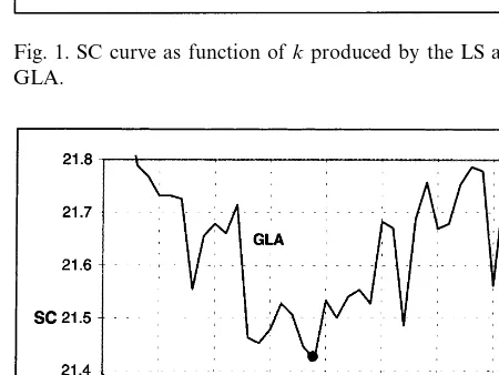
Fig. 1. SC curve as function ofkproduced by the LS and the GLA.
In the present study, we consider the role of the clustering algorithm in numerical taxonomy. In particular, we want to answer two questions in this context. First, we compare the performance of the two clustering clustering algorithms mea-sured by the best values of the cost function. Second, it is by no means evident that different algorithms would produce similar results. Even if the values of the cost function were similar, it would not imply that the classifications were the same. This is because the algorithms may con-verge to different local minima with the same value. The cost function, on the other hand, guides the clustering algorithm to find certain types of solution.
We use the classification of 5313 strains of bacteria belonging to the Enterobacteriaceae fam-ily as a case study. In particular, we discuss two efficient clustering algorithms, the generalized lloyd algorithm (GLA) (Linde et al., 1980); and the local search (LS) (Fra¨nti et al., 1998; Fra¨nti and Kivija¨rvi, 2000). The GLA has been applied to the Enterobacteriaceae data by Gyllenberg et al. (1997a), where a classification into 69 classes was obtained.
Local search (LS) is one alternative amongst effective clustering algorithms based on optimiza-tion techniques. It has originally been applied to the construction of the codebook in vector quan-tization. In this context, it has turned out to be Fig. 2. SC curve from the interesting range. The black dots
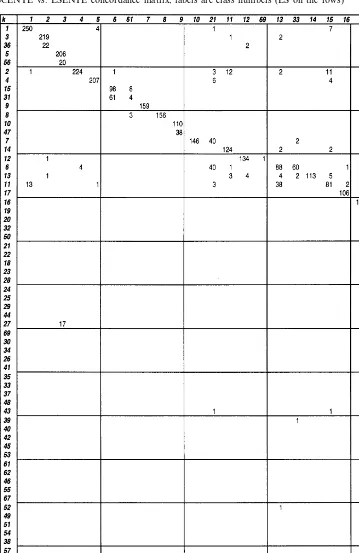
Table 1
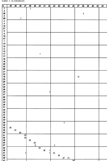
Table 1 (Continued)
Fig. 4. Frequency histograms of the distortion values for the GLA- and LS-classifications. Distortion intervals (length of 0.5) are onx-axis and counts ony-axis.
Fig. 5. Cluster size histograms of the GLA- and LS-classifications. Size intervals (length of 10) are onx-axis and counts ony-axis.
very competitive finding extremely effective code-books in reasonable time (Fra¨nti and Kivija¨rvi, 2000). In vector quantization, the LS has been applied using the mean square error as the cost function. In the present paper, we give necessary modifications for the method in order to apply stochastic complexity as the cost function in the LS. Other well known methods that could be for the clustering by SC are for example genetic al-gorithms (Fra¨nti et al., 1997) and simulated an-nealing (Zeger and Gersho, 1989) but the simplicity of the LS makes it more suitable with the SC.
2. The classification problem
LetS={x¯(l)
l=1, 2, …,t} be a set of telements (feature vectors) of the form x¯(l)
=(x1 (l),
x2 (l), …,
xd
(l)); x
i
(l)
{0, 1} for all l{1, 2, …, t}, i{1, 2, …,d}, dbeing the dimension of the vectors. Our task is to determine a classification of S into k
classes so that the cost of the classification is
minimal. We must consider three sub problems when generating a classification,
1. selecting a measure for the cost of the classification;
2. determining the number of classes used in the classification; and
3. selecting a suitable clustering algorithm. These sub problems are interrelated but there are still many degrees of freedom in each selec-tion. The choice of the number of classes has been discussed in (Gyllenberg et al., 1997b). In this paper, our main interest is to understand how the clustering algorithm itself affects the outcome.
Table 2
Distance between the classifications according to Eq. (5)
CFARM SCENTE LSENTE
* CFARM
SCENTE 1441.0 *
Table 3
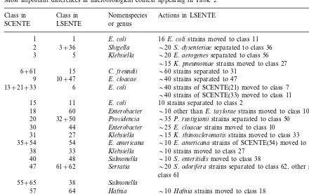
Most important differences in microbiological context appearing in Table 2 Class in Nomenspecies
Class in Actions in LSENTE
LSENTE
SCENTE or genus
1 1 E.coli 16E.colistrains moved to class 11 Shigella
3+36 20S.dysenteriaeseparated to class 36 2
Klebsiella
3 5 20E.aerogenesseparated to class 56
15K.pneumoniaestrains moved to class 27 6+61 15 C.freundii 60 strains separated to 31
E.cloacae
10+47 40 strains separated to 47
9
E.coli
13+21+33 6 40 strains of SCENTE(21) moved to class 7
40 strains of SCENTE(33) moved to class 11 E.coli
15 11 10 strains separated to class 2
Enterobacter
60 10 other thanE.tayloraestrains moved to class 10
18
Pro6idencia
20 32+50 35P.rustigianiistrains separated to class 50 Enterobacter
44 25E.cloacaestrains moved to class 10 30
31 27 Klebsiella 15K.rhinoscleromatisstrains moved to class 33 E.americana
54 10E.americanastrains of SCENTE(54) moved to class 36 35+54
33
38 Klebsiella 10 strains moved to class 27 48
40 Salmonella 10S.enteritidismoved to class 38 Serratia
61+62 20S.odoriferastrains separated to class 62, other strains separated to 47
57 10Hafniastrains moved to class 18
+Koserella Trash classes
67+68 68
Trash class
69 Single strain joined to class 12
2.1. Stochastic complexity
We describe mathematically a classification of strains with d binary (0 or 1) features into k
classes by the numbers
l
whereljis the relative frequency of strains in the
jth class and uijis the relative frequency of 1 s in the ith position in the jth class. The centroid of the jth class is the vector (u1j, u2j, …, udj). The
(Dybowski & Franklin, 1968; Willcox et al., 1980)
As a statistical model of the classification we, therefore, choose the distribution
p(x)=%
j and uijbeing the parame-ters of the model. We emphasize that this statisti-cal representation is simply a mathematistatisti-cally convenient way of defining the classification model and it does not imply any randomness in the data.
It was shown by Gyllenberg et al. (1997b) that the stochastic complexity SC of a set of t strains with respect to the above model is
is the number of strains in classjwithith feature equal to one. The two first terms in (Eq. (3)) describe the complexity of the classification and the third term, the complexity of the strains with respect to the classification.
To classify the feature vectors by minimizing stochastic complexity, we apply the Shannon-codelength instead of the L2-distance that was originally used by Linde et al. (1980) (see also Gersho and Gray, 1992)
CL(x,Cj)
j and is called weight of the class. Minimization of expression Eq. (4) clearly mini-mizes the expression Eq. (3).
2.2. The generalized Lloyd algorithm
Given the number k of classes, the GLA for minimizing SC works as follows,
Step 1. Drawkinitial centroids randomly from the set of input vectorsS.
REPEAT TEN TIMES.
Step 2.1. Assign each input vector to the closest cluster centroid with L2-distance. Step 2.2. Calculate new cluster centroids. REPEAT.
Step 3.1. Assign each input vector to the closest cluster centroid with Formula 4. Step 3.2. Calculate new cluster centroids and class weights, and evaluate the distortion with Eq. (3).
UNTIL no more improvement in distortion value.
The algorithm (also known as LBG or k -means) (McQueen, 1967; Linde et al., 1980) starts with an initial solution, which is iteratively im-proved using the two step procedure. In the first step (step 2.1), the data objects are partitioned into a set ofkclusters by mapping each object to the closest cluster centroid. In the second step
(step 2.2), the centroids and the weights of the clusters are updated. We represent the centroids by floating point numbers (i.e. the components of a centroid are the relative frequencies of one-bits). The process is first repeated ten times using the L2-distance for the following reasons, (i) an initial solution is needed for calculating the cluster weights; (ii) the CL-distance is highly dependent of the quality of the initial solution; and, there-fore, we need more than one iteration with L2; (iii) the use of the L2-distance reduces the compu-tational load of the algorithm. In the next steps (steps 3.1 and 3.2), the GLA is performed using the CL-distance. This process is repeated as long as improvement is achieved in the cost function value (SC).
Another problem is connected with the so-called orphaned centroids (also known as the empty cell problem). Orphaned centroids have no vectors assigned to them in the steps 2.2 and 3.2 of the algorithm. The orphaned centroids must be eliminated, otherwise the number of non-empty classes would be less than the prescribed k. Whenever an orphaned centroid occurs, it is re-placed by splitting an existing class having the greatest distortion. The centroid of the new class is taken as the vector with the greatest distance to the original centroid of the split class, as proposed by Kaukoranta et al. (1996). The GLA iterations then continue with the modified set of centroids. A significant benefit of the GLA is its fast operation. On the other hand, the main drawback of the GLA is that it is only a simple descent method and, therefore, converges at the first local minimum. The result depends strongly on the quality of the initial solution. An easy way to improve the method is to repeat the algorithm for several different initial solutions and select the one with minimal value of the cost function (Eq. (3)). In the following, we use this approach.
2.3. The local search algorithm
to use SC as the cost function instead of the MSE. The algorithm forms an initial classification and iteratively improves it by applying a randomizing function, and the GLA. Given the number of classesk, the control flow of the LS method is as follows.
Step 1. Drawkinitial centroids (from the input data) randomly.
Step 2. Assign each input vector to the closest cluster centroid.
ITERATET times
Step 3.1. Replace a randomly chosen class. Step 3.2. Re-assign each input vector accord-ing to the changed class.
Step 3.3. Perform two iterations of the GLA using L2 distance.
Step 3.4. Evaluate the cost function value Eq. (3).
Step 3.5. If the modifications improved the classification, accept the new classification. Otherwise restore the previous classification. Step 4. Perform the GLA using the CL-crite-rion Eq. (4) for the final solution.
The initial classification is generated as in the GLA, i.e. the algorithm selects items randomly as the class representatives (HMO, hypothetical mean organism). The rest of the strains are as-signed to the closest class representative according to the L2-distance. A new trial classification is then generated by making random modifications to the current one, a randomly chosen class is made obsolete and a new one is created by select-ing any sample strain as the new HMO. The resulting classification is improved by the GLA. This generates changes in the class representatives of the trial classification. The trial classification is accepted if it improves the cost function value, which is the SC.
The advantage of the LS over the GLA is that it makes global changes to the clustering struc-ture, and at the same time performs local fine tuning towards a local optimum. In our practical tests, we let the algorithm run for 5000 iterations in total, and two iterations of the GLA is applied for each trial solution. This gives us a good balance between the global changes in the cluster-ing structure and the local modifications in the classification. During the search (step 3), we do
not use the Shannon-codelength (CL) when as-signing the vectors to the clusters because it is problematic with the chosen randomization func-tion. It is also much slower and does not enhance the performance according to our tests. The final solution, however, is fine-tuned by the GLA using the CL-criterion. The steps 1 – 3 of our LS-al-gorithm, thus, form a preprocessing phase for the SC-clustering.
2.4. Number of classes
The optimum number of classes is, by defini-tion, the value k* at which the overall minimum of SC is attained. A straightforward solution is, therefore, to apply the GLA and the LS for every reasonable number of classes (1 – 110). From the results of each fixed k, we take the one with minimal stochastic complexity. The LS was per-formed only once with the iteration count 5000 whereas the GLA was repeated 50 – 200 times.
2.5. Difference between the classifications
There are basically two ways for measuring the difference between classifications, either we mea-sure the smallest number of modifications (usually set operations) that are needed to make the two classifications equal, or we count some well defined differences between them (Day, 1981). Modifications and differences can be defined in various ways and they should be chosen carefully to suit the application. We illustrate the difference between two given classifications denoted byP%=
{C%1, …, C%k%} and P¦={C¦1, …, C¦k¦}. The
Con-cordance matrixMis ak%byk¦matrix with entry
Mij defined as the number of elements in C%i S C¦j. The distance between two classifications can now be calculated from the concordance matrix by
alternative is to trust a domain expert, here to a microbiologist, and let him judge the classifica-tions P% and P¦ against the best state of art knowledge of the taxonomy of the strains. This evaluation gives us insight of the usability of our algorithms and proximity functions.
3. Application to classification of Entero-bacteriaceae
The data set (called ENTE) consists oft=5313 strains of bacteria belonging to the Enterobacteri-aceae family. The strains have been isolated dur-ing the years 1950 – 1988 and identified by CDC in Atlanta, Georgia (Farmer et al., 1985). The material consists of 104 nomenspecies. We refer to nomenspecies classification as CFARM (SC/t=
23.12). Each strain is characterized by a binary vector of d=47 bits representing outcomes of biochemical tests. For a detailed description of the material, see Farmer et al. (1985).
4. Results
Gyllenberg et al. (1997a) calculated the SC min-imizing classification of ENTE using GLA and obtained a classification into 69 classes with the SC-value 21.42. This classification is called SCENTE. At least 20 repetitions were run for eachk, the best candidates were inspected 50 – 200 times. Thus, the total running time for SC-mini-mization was very long, a few days with an effi-cient computer, although the partitioning of one candidate is a quick operation (few minutes). The LS is about 100 – 200 times slower than the GLA for a single classification. The LS, on the other hand, is rather independent of the initialization and, therefore, only a single run is enough whereas the GLA, as mentioned above, had to be repeated 50 – 200 times. This balances the compu-tational differences of the methods.
As the first step, we classified the material with the LS for all k-values from 1 to 110 and com-pared the SC-values with the ones obtained previ-ously by the GLA. They both give the minimum SC-values approximately in the same range (see
Fig. 1). The curve for the LS is very flat for
k-values in the range k=60–72 (see Fig. 2). The LS found SC values from 21.28 to 21.33 with the mean 21.30 and S.D. 0.016 for these k-values. This means that there are several values of k
which produce almost equally good classification in the sense of minimizing SC. The corresponding SC-values for the GLA vary from 21.42 to 21.72 with the mean 21.53 and S.D. 0.094.
We studied the methods more closely on the previously found minimum point (k=69). The results obtained by the LS have less variation and are consistently better than the results of GLA (Fig. 3). For example, the LS always produced classification with smaller SC-value than the best SC-value obtained by the GLA. The correspond-ing SC-values for the LS vary from 21.27 to 21.35, and for the GLA from 21.51 to 22.18.
As a second step, we compared the two classifi-cations by producing the class concordance ma-trix for them. We focus on differences between the LS and GLA classifications, see Table 1. The rows of the matrix stand for the classes of the LS-so-lution and the columns for the classes of the GLA-solution. Note that the class indices are se-lected by the size of the classes in descending order. If the two classifications resemble each other there is a good concordance between some corresponding pairs of classes from LS and GLA. To increase the level of illustration, we have ad-ditionally arranged the rows and columns of the matrix such that the greatest matrix-elements ap-pear on the diagonal. The total number of ele-ments of a particular class appear as row/column sum.
Table 1 shows that the class with index 6 of LSENTE consists of 303 strains which are scat-tered over classes 13 (88 strains), 33 (60), 21 (40), 23 (6), 4 (4), 11 (1), 41 (1), 42 (2) and 16 (1) of SCENTE. The joining of the three classes 13, 33 and 21 in other classification is natural because these represent the species E. coli. Similar phe-nomena can be found for example inE.americana
the LSENTE classification, theC.freundii strains are scattered over two major classes (15, 31).
Fig. 4 shows the distribution of the distortion values (average Hamming distance from HMO) for the two classifications. The distortion values of both LSENTE and SCENTE resemble normal distribution. Fig. 5 demonstrates the class size distributions, first bar represents number of classes having size in range 1 – 10, and second 11 – 20 and so forth. There are some small classes in both classifications and they are likely due to some badly fitting vectors in data (i.e. trash).
As a third step, we calculated the distance D
between the classifications and CFARM. The re-sults of Table 2 show that the LSENTE and SCENTE classifications, whose stochastic com-plexities were smaller, are closer to each other than to CFARM. On the other hand, the LSENTE and SCENTE classifications are almost as far from CFARM.
As a fourth step, we compared the classifica-tions made by the classification algorithm to the expert class (CFARM). Our data had scientific names (104 nomenspecies) and identification numbers attached to the vectors. This allows us to analyze how well the obtained classifications conform to the currently established classification of Enterobacteriaceae. Most of the data repre-sent species of E. coli, hence we concentrate on this part.
The E. coli strains tend to divide into two groups. These correspond to the so-called active and inactive E. coli (Farmer et al., 1985). The LSENTE classes 6, 13, 14 represent inactive E.
coli group and the classes 1, 2, 4, 7, 17, 39, 43 active group. Similarly, E. coli is divided into two remote groups of SCENTE classes 15, 21, 33, 13, 11 and 42, 41, 4, 10, 5, 16, 1. We noted before that LSENTE class 6 was scattered to many classes in SCENTE (mainly 13, 21, 33). It seems that LS has managed to classify the inac-tive group of E. coli more efficiently. On the other hand, the active E.coli’s are classified simi-larly in both classifications. We have listed most microbiologically relevant differences in Table 3. We find these phenomena similar to the findings of Gyllenberg et al. (1998) Gyllenberg et al. (2000).
5. Conclusions
We have compared two clustering algorithms using a taxonomic problem in microbiology as a case study. One of the algorithms is the classical GLA algorithm whereas the other applies an effi-cient local search strategy to improve the classifi-cation. A general observation is that the classifications do not differ radically when evalu-ated by SC. The LS was somewhat more effec-tive than GLA.
The comparison of the classifications reveals several interesting facts. A class may be split into two or more classes in the classifications ob-tained by GLA and LS. The splitting of the clusters is usually reasonable from a microbio-logical point of view.
In spite of the different strategies in the GLA and the LS, the distributions of the class sizes of the two classifications look similar. This is most likely due to the data used in this experiment. It turned out that the repeated use of GLA with random initial solutions can produce good clas-sifications. Iterative optimization techniques like LS are, however, more reliable in the sense that they search more systematically for the global optimum. To demonstrate this, we calculated the histogram of SC values, which shows that results of LS are more biased to better SC-values. Even though the implementation of the LS and the GLA is a relatively easy task, we were con-fronted by some practical issues, which need spe-cial consideration. These include the case when a cluster consists of a single strain only. In this case, vectors are seldom mapped to this new cluster when the entropy distance (6) is used. The use of the L2-distance solves this problem. The overall evaluation of the preference of the two classifiers favor the LS because the GLA is more dependent on setting of the initial centroids, and as shown above, the LS will more likely produce a good solution.
Acknowledgements
This work has been supported by the Academy of Finland, The Swedish Natural Sci
ence Research Council (NFR) and by the Knut and Alice Wallenberg Foundation.
References
Bock, H.-H., 1996. Probability models and hypothesis testing in partitioning cluster analysis. In: Arabie, C.P., Hubert, L.J., De Soete, G. (Eds.), Clustering and Classification. World Scientific, Singapore, pp. 377 – 453.
Day, W.H.E., 1981. The complexity of computing matrix distances between partitions. Math. Soc. Sci. 1, 269 – 287. Dybowski, W., Franklin, D.A., 1968. Conditional probability
and identification of bacteria. J. Gen. Microbiol. 54, 215 – 229.
Farmer, J.J., Davis, B.R., Hickman-Brenner, F.W., McWhorter, A., Huntley-Carter, G.P., Asbury, M.A., Rid-dle, C., Wahten-Grady, H.G., Elias, C., Fanning, G.R., Steigerwalt, A.G., O’Hara, C.M., Morris, G.K., Smith, P.B., Brenner, D.J., 1985. Biochemical identification of new species and biogroups of Enterobacteriaceae isolated from clinical specimens. J. Clin. Microbiol. 21, 46 – 76. Fra¨nti, P., Kivija¨rvi, J., 2000. Randomized local search
al-gorithm for the clustering problem. Pattern Analysis and Applications 3, in press.
Fra¨nti, P., Kivija¨rvi, J., Kaukoranta, T., Nevalainen, O., 1997. Genetic algorithms for large scale clustering problems. Comput. J. 40 (9), 547 – 554.
Fra¨nti, P., Kivija¨rvi, J., Nevalainen, O., 1998. Tabu search algorithm for codebook generation in vector quantization. Pattern Recognition 31 (8), 1139 – 1148.
Gersho, A., Gray, R.M., 1992. Vector Quantization and Signal Compression. Kluwer Academic Publishers, Dordrecht. Gyllenberg, H.G., Gyllenberg, M., Koski, T., Lund, T.,
Schin-dler, J., Verlaan, M., 1997a. Classification of Enterobacteri-aceae by minimization of stochastic complexity. Microbiology 143, 721 – 732.
Gyllenberg, M., Koski, T., Verlaan, M., 1997b. Classification of binary vectors by stochastic complexity. J. Multivariate Anal. 63, 47 – 72.
Gyllenberg, H.G., Gyllenberg, M., Koski, T., Lund, T., 1998. Stochastic complexity as a taxonomic tool. Comput. Meth-ods Programs Biomed. 56, 11 – 22.
Gyllenberg, H.G., Gyllenberg, M., Koski, T., Lund, T., Schin-dler, J., 2000. Enterobacteriaceae taxonomy approached by stochastic complexity. Quant. Microbiol. 1, 157 – 170. Kaukoranta, T., Fra¨nti, P., Nevalainen, O., 1996. Reallocation
of GLA codevectors for evading local minima. Electron. Lett. 32, 1563 – 1564.
Linde, Y., Buzo, A., Gray, R.M., 1980. An algorithm for vector quantizer design. IEEE Trans. Commun. 28, 84 – 95. McQueen, J.B., 1967. Some methods of classification and
analysis of multivariate observations. Proceedings of Fifth Berkeley Symposium of Mathematical Statistics Probabil-ity, 1, Berkeley, CA, pp. 281 – 296.
Rissanen, J., 1989. Stochastic Complexity in Statistical Inquiry. World Scientific, Singapore.
Willcox, W.R., Lapage, S.P., Holmes, B., 1980. A review of numerical methods in bacterial identification. Antonie Leeuwenhoek 46, 233 – 299.
Zeger, K., Gersho, A., 1989. Stochastic relaxation algorithm for improved vector quantiser design. Electron. Lett. 25, 896 – 898.