Original scientific paper UDC 336.27:330.35
Public debt and growth: evidence from Central,
Eastern and Southeastern European countries
*Anita Čeh Časni
1, Ana Andabaka Badurina
2, Martina Basarac Sertić
3Abstract
The aim of this paper is to quantify the long run and short run relationship between debt and economic activity in Central, Eastern and Southeastern European countries. In order to investigate the impact of public debt on economic growth, the paper uses pooled mean group estimator (PMG) for the period between 2000 and 2011. A battery of panel unit root as well as panel cointegration tests is used prior to performing the dynamic panel analysis based on PMG estimator. According to the empirical results, in the long-run debt significantly influences the GDP growth having a negative sign as expected and pointing out that government gross debt lowers the GDP growth. In the short run, debt has statistically significant negative influence on the GDP growth as well, controlling for other determinants of growth (trade openness, total investment and industry value added). Designing policy frameworks that encourage export, promote industrial development and create better environment for long-term investment should foster sustainable growth. Therefore, we find that a credible fiscal consolidation strategy is needed combined with policies to promote lasting growth in order to reach debt-stabilizing levels.
Key words: debt, economic growth, pooled mean group estimator, European countries
JEL classification: C33, F43, H63
* Received: 20-11-2013; accepted: 06-06-2014
1 PhD, Teaching and Research Assistant, University of Zagreb, Faculty of Economics and Business, Trg J. F. Kennedyja 6, 10000 Zagreb, Croatia. Scientific affiliation: business statistics, multivariate statistics, econometrics applications in macroeconomics. Tel: +385 1 2383 353. E-mail: aceh@efzg.hr. Personal website: http://www.efzg.unizg.hr/aceh.
2 PhD, Teaching and Research Assistant, University of Zagreb, Faculty of Economics and Business, Trg J. F. Kennedyja 6, 10000 Zagreb, Croatia. Scientific affiliation: macroeconomics, public debt management. Tel: +385 1 2383 229. E-mail: aandabaka@efzg.hr. Personal website: http://www.efzg.unizg.hr/default.aspx?id=2771.
3 PhD, Research Assistant, Croatian Academy of Sciences and Arts, Strossmayerov trg 2, 10000 Zagreb, Croatia. Scientific affiliation: economic development, macroeconomic drivers, economic convergence, dynamic analysis. Tel: +385 1 4895 105. E-mail: mbasarac@hazu.hr.
1. Introduction
Global economic and financial crisis triggered the ongoing sovereign debt crisis in Europe and raised the issue of public debt sustainability. The sustainability of government finance was compromised by the fall in public revenues owing to a sharp fall in output as well as pronounced increase in fiscal risk due to exchange-rate movements and private debt overhang. Given the scarce empirical research on this subject, there is a need to further explore the debt-growth relationship and highlight the effect of public debt on economic activity.
The interaction between public debt and economic growth is rather complex because public debt influences the economic growth dynamics and the economic growth rates impact the size of public debt. Higher rates of economic growth facilitate carrying public debt burden (Cantor and Packer, 1996). Public debt sustainability depends on its ability to raise revenue which decreases when economy experiences a downturn. The private sector default has adverse effect on economic activity and increases public debt when private borrowing is backed by discretionary fiscal policy (Cecchetti et al., 2011).
In theory, the effects of government debt on economic growth can be ambiguous. Public debt can both stimulate the economy and hinder the economic growth. The size and structure of public debt really matter as well as the allocation of borrowed funds. According to the golden rule of public finance over the economic cycle, the government should borrow only to invest and not to fund current spending. This rule protects the investment spending while targeting over the cycle allows automatic stabilizers to work without jeopardizing long-term fiscal sustainability (Keiko, 2007). In other words, debt should be used only to finance productive government expenditures that increase public capital formation and promote strong and sustainable economic growth. However, during the latest financial and economic crisis the fiscal stimulus was needed in order to support financial system and to mitigate the spillover effects to the real economy.
The recent crisis highlighted the importance of interest rates channel through which public debt can affect financial stability, private spending and consequently economic growth. Higher share of short-term public debt increases the rollover ratio4 and refinancing needs while putting greater pressure on short-term interest
rates. Thus, issuing high amounts of short-term debt in the money market might increase the influence of government financing on interest rates and complicate the steering of nominal interest rates by monetary authorities (Hoogduin et al., 2010). IMF (2011) finds that maintaining low rollover profile makes it easier to absorb the realization of contingent liabilities and financing impact of reduced tax receipts during recession and provides several other benefits: it (i) reduces the risk that an
4 Indicator for refinancing-risk defined as short-term debt stock of the previous year plus maturing
investor flight will drive up yields; (ii) reduces debt servicing costs as a consequence of a deterioration in sovereign creditworthiness; (iii) provides resilience where the exchange rate regime constrains policy choices. During the crisis both the rollover ratio and the public debt-to-GDP ratio increased considerably while demand for government bonds was severely reduced. When credit ratings deteriorate, market participants demand a higher interest rate risk premium pushing sovereign bond yield spreads higher and affecting long-term interest rates.
According to the neoclassical model the crowding-out effect occurs when government borrowing drives up interest rates and causes subsequent reduction in private spending. On the contrary, increase in debt-financed government expenditures which stimulate demand for goods and services in turn crowds-in private investment. Woodford (1990) emphasizes the positive liquidity effects of government borrowing and suggests that welfare could be increased by a permanent increase in the level of the public debt.Empirical research supports both crowding-out and crowding-in as well as mixed results. The recent studies suggest that a nonlinear relationship between public debt and economic growth should be described by inverted U-shaped curve with the certain turning point beyond which increase in public debt has significant and negative impact on growth (Reinhart and Rogoff, 2009; Checherita and Rother, 2010; Baum et al., 2013). The debt turning point is usually expressed as the threshold value of debt-to-GDP ratio indicating that governments should keep their public debt below the estimated value to foster economic growth and development.
The size of public debt affects the economic activity and the effectiveness of fiscal policy measures. IMF (2008) finds that the concerns about public debt sustainability could threaten the effectiveness of fiscal stimulus by increasing real interest rates and lowering output multipliers to a point at which discretionary fiscal policy would do more harm than good. Cecchetti et al. (2011) conclude that, at low and moderate levels, public debt improves welfare and enhances economic growth and stability. High and excessive public debt, on the other hand, inhibits growth and increases volatility. The purpose of this paper is to analyse the long run and short run impact of public (gross government) debt on GDP growth. The hypothesis of the paper is that public debt has adverse effect on economic growth. Almost all Central and Southeastern European countries5 are included in the analysis during the period between 2000
5 Although these countries share some common features, we must emphasize that they are rather
heterogeneous considering different levels of economic development and integration with the EU (EU member states, candidate and prospective candidate countries). The common feature of countries engaged in a transition process was the need to encourage private investment in order to build up capital stock taking into account low domestic savings. The abolition of capital controls during the process of EU accession paved the way for significant capital inflows especially foreign direct investment. The economic growth was mainly driven by private consumption (except Hungary and Croatia) and investment although to a less extent, while net exports had negative impact on growth especially in countries with fixed or tightly managed nominal exchange rate (Sándor and Martin, 2010).
and 2011. Previous empirical studies have been based either on euro area (Baum et al., 2013; Checherita and Rother, 2010) or selected group of developing countries (Imbs and Rancire, 2005; Pattillo et al., 2011). Furthermore, the empirical analysis in this paper differs from previous research regarding applied methodology. Namely, in order to investigate the impact of public debt on economic growth, pooled mean group estimator (PMG) in a manner of Pesaran, Shin and Smith (1999) is used. Likelihood-based PMG estimator constrains the long-run elasticity to be equal across all countries, which yields efficient and consistent estimates when homogeneity restriction is true, which is tested using Hausmann homogeneity test. Also, before performing the empirical analysis based on PMG estimator, a battery of panel unit root tests as well as panel cointegration tests is conducted with the aim of testing statistical properties of the variables of interest.
The results show that in the long-run, debt significantly influences the GDP growth, it has a negative sign as expected, pointing out that general government gross debt lowers the GDP growth. In the short run, debt has statistically significant negative influence on GDP growth as well. Furthermore, according to estimated model, all three control variables (trade openness, total investment and industry value added) have statistically significant influence on GDP growth in the short run, with economically meaningful signs, stressing their positive influence on GDP growth. The contribution of our paper stems from the above mentioned and from the empirical results.
Given the empirical results for the specific group of countries, we find that a credible fiscal consolidation strategy is needed combined with policies to promote lasting growth in order to reach debt-stabilizing levels. Although the fiscal adjustment measures can have contractionary effect on private demand and output growth in the short run according to Keynesian view, a credible strategy implemented at a right pace can also have a positive indirect effect on aggregate demand through an improvement in expectations if the measures taken are designed to permanently reduce the share of government in GDP and taxation in the future (Hellwig and Neumann, 1987).
Fiscal consolidation policy implications may differ given the country-specific economic features. The countries should focus on restraining public expenditures while preserving public capital formation and other expenditures with strong positive spillovers, especially those with sizable government sector. However, there is a need to balance both tax and spending measures in order to achieve appropriate fiscal adjustment. Moreover, tax measures should focus on improving tax governance and tax base-broadening reforms6 rather than increasing tax rates. Finally, carefully
designed fiscal adjustment offers an opportunity to improve the quality of government spending as well as the structure of the tax system (Carnot, 2013).
The remainder of the paper is organized as follows. In Section 2 the literature review is presented. Applied research methodology and date are described in Section 3. Section 4 presents the empirical data and analysis. The main results of the econometric analysis based on a pooled mean group estimator are given in Section 5. Section 6 concludes.
2. Literature review
The current sovereign debt crisis has forcefully revived the academic and policy debate on the economic impact of public debt (Baum et al., 2013). Nevertheless, the empirical studies estimating the effect of public debt on economic growth remain scarce and limited (Schclarek, 2004; Baum et al., 2013).
In this section, we highlight the papers that focus on gross government debt and use panel data analysis as preferred estimation technique. Checherita and Rother (2010) examine the average impact of government debt on per-capita GDP growth in 12 euro area countries during the 1970-2011 period using panel fixed-effects corrected for heteroskedasticity and autocorrelation. They find a non-linear impact of debt on growth with a turning point, beyond which the government debt-to-GDP ratio has a deleterious impact on long-term growth, at about 90-100% of GDP. Moreover, confidence intervals for the debt turning point signify that the negative growth effect of high debt may start from levels of around 70-80% of GDP. Simultaneously, there is evidence that the annual change of the public debt ratio and the budget deficit-to-GDP ratio are negatively and linearly associated with per-capita GDP growth. The other explanatory variables through which public debt is found to have an impact on economic growth rate are private saving, public investment, total factor productivity and sovereign long-term nominal and real interest rates.
A similar conclusion on the relationship between debt and growth can be found in Cecchetti et al. (2011). Namely, they analyse 18 OECD countries from 1980 to 2010, and their empirical results point out that when government debt goes beyond 85% of GDP, it becomes a drag on economic growth.
Furthermore, several other papers use a dynamic threshold panel methodology in order to analyse the non-linear impact of public debt on GDP growth. For example, Kumar and Woo (2010) analyse the impact of high public debt on long-run economic growth for a panel of 38 advanced and emerging economies in the period 1970–2007. Therefore, they utilize a variety of estimation methods, such as pooled OLS, robust regression between estimator, fixed effects panel regression, and system GMM. Their empirical results suggest an inverse relationship between initial debt and subsequent growth, controlling for other determinants of growth:
initial income per capita, average years of schooling, financial market development, inflation, banking crisis and fiscal deficit.
Furthermore, Reinhart et al. (2012) in their historical analysis identify 26 episodes where (gross central government) debt to GDP ratios exceeds 90% of GDP since 1800. The authors find that in 23 of these 26 episodes, countries experienced lower growth than the average of other years.
On the contrary, Baum et al. (2013) focus on 12 euro area countries for the period 1990-2010 and their empirical results suggest that the short run impact of debt on GDP growth is positive and highly statistically significant, but decreases to around zero and loses significance beyond public debt-to-GDP ratios of around 67%. However, for debt-to-GDP ratios above 95%, additional debt has a negative impact on economic growth.
Apart from the above mentioned papers, various studies explore the relationship between external debt and growth. For example, Pattillo et al., (2011) examine the impact of external debt on growth using panel data for 93 developing countries. Their findings suggest that the average impact of debt becomes negative at about 160-170 percent of exports or 35-40 percent of GDP and the marginal impact of debt at about half of these values. Another contribution is provided by Imbs and Ranciere (2005). Namely, the authors focus on measures of gross external debt, for a sample of 87 developing economies (that includes low and middle income according to the World Bank classification), over the period 1969-2002. They estimate growth specification using ordinary least squares, fixed effects, and a GMM system estimator. According to their results, there is no robust linear evidence of a negative relationship between debt and growth in the full sample. Furthermore, on average, debt overhang occurs when the face value of debt reaches 55 to 60 percent of GDP or 200 percent of exports, or when the present value of debt reaches 35 to 40 percent of GDP or 140 percent of exports. Then, initial debt tends to be associated with subsequently low growth. They also investigate the role of institutions and find that institutions do matter for debt and growth. Finally, the authors find that investment collapses in the overhang zone, and the conduct of economic policy deteriorates observably.
Cordella et al. (2010) also investigate the effect of external debt rise and institution quality on per capita growth. Their findings suggest that countries with good policies and institutions face overhang when net present value of debt rises above 20–25 percent of GDP. However, debt becomes insignificant when it rises above 70–80 percent of GDP. According to authors, in economies with bad policies and institutions, overhang and irrelevance thresholds seem to be substantially lower (10–15 and 15–35 percent of GDP, respectively), but the results are not robust to alternative specifications.
3. Research methodology and data
In this part of the paper the impact of debt on GDP growth using panel data analysis is explored. Empirical analysis is performed on a sample of 147 European countries
in the period between 2000 and 20118.
The literature on dynamic and co-integrated panels rapidly evolved over the past decade, proposing a number of estimators that solve different econometrics issues. In this paper we rely on recent papers by Pesaran, Shin and Smith (1997, 1999) that offer two important techniques to estimate non-stationary dynamic panels in which the parameters are heterogeneous across groups, namely the mean group (MG) and pooled mean group (PMG) estimators. Precisely, Mean Group estimator (MG) which is based on estimating N time-series regressions and averaging the coefficients (Pesaran and Smith, 1995), and PMG estimator which is a combination of pooling and averaging of coefficients (Pesaran et al., 1999) are used. Taking into account that analysed 14 economies are different with the respect to their economic policy, the two mentioned dynamic panel models are estimated9.
Among them, pooled mean group estimator (PMG) proposed by Pesaran et al. (1999) is especially attractive, since it allows the short run responses to be flexible and unrestricted across groups, while imposing restrictions by pooling individual groups in the long run. In other words, likelihood-based PMG estimator constrains the long-run elasticity to be equal across all panels, which yields efficient and consistent estimates only when homogeneity restriction is indeed true. Furthermore, when N is rather small, like in our case, PMG estimator is less sensitive to outliers (Pesaran et al., 1999) and can simultaneously correct the serial autocorrelation problem and the problem of endogeneous regressors by choosing appropriate lag structure for both: dependent and independent variables. Since, the focus of this paper is the impact of public debt on economic growth in the long and in the short-run, in order to capture that relationship empirically, the following equation is estimated:
gdp_growthit = γ0i + γ1idebtit + γ2iopennessit +γ3iinvestmentit +
+ γ4iindustryit + εit, i = 1, 2, ..., N; t = 1, 2, ..., T (1)
7 Central, Eastern and Southeastern European countries: Albania, Bosnia and Herzegovina, Bulgaria,
Croatia, the Czech Republic, Germany, Hungary, Macedonia, Montenegro, Poland, Romania, Serbia, Slovakia and Slovenia.
8 The analysis is performed on yearly data and panel consisted of 14 countries. Also, the empirical
analysis was conducted using EViews 7 and Stata 12 software.
9 OLS estimators are super-consistent in the case of co-integrated variables, but they are based on
strong homogeneity assumptions among countries by imposing single slope coefficient in pooled estimation, which is inappropriate for this study regarding potential country heterogeneity. This is the reason for using PMG estimator instead of traditional panel techniques.
where gdp_growth is the annual percentage GDP growth rate, debt is the general government gross debt expressed in percentages of GDP, openness represents trade openness (as a percentage of GDP), investment is the ratio of total investment (as a percentage of GDP) and industry is expressed as an annual percentage growth rate. Error term capturing the effects of unexpected shocks to gdp_growth is denoted by εit. The subscripts i and t denote country and time respectively, suggesting an
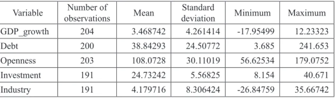
unbalanced panel. Construction of these variables is standard (description of the data is given in Table 1 in the Appendix). As far as the data sources are concerned, in the empirical analysis the World Development Indicators and the World Economic Outlook were used. Descriptive statistics of variables used in the analysis is given in Table 2 in Appendix.
Also, in this framework it is assumed that in the short-run, GDP growth differs across countries. This assumption is hereby implemented by using conventional statistical criteria and determining lag length of each variable. Furthermore, an important issue that needs to be dealt with in econometric analysis is the dynamic structure of GDP growth model, assuming that certain economic aspects prevent immediate adjustment of GDP to changes in its fundamental determinants. Accordingly, the first and necessary step of the empirical analysis was to choose the lag order of ARDL model by applying the Schwarz information criterion10.
Even though there was no clear evidence of a most common representation, after choosing a country specific lag order of the ARDL model by applying the SBC information criterion, the preferred specification for the whole sample of analysed countries was an autoregressive distributed lag ARDL (1,0,0,0,0) model:
gdp_growthit = δi + β10idebtit + β20iopennessit + β30iinvestmentit +
+ β40iindustryit + γigdp_growthi,t–1 + ηit (2)
That is, GDP growth is lagged once, whereas general government gross debt, trade openness, the ratio of total investment and industry are given in levels.
According to Engle and Granger (1987) if the variables are I(1) and co-integrated, the error term is an I(0) process for all countries (i). Furthermore, co-integrated variables show great responsiveness to any deviation from long-run equilibrium, so this feature implies an error correction reparametrization of equation (2) such as:
Δgdp_growthit = φi(gdp_growthi,t–1 – γ0i – γ1idebtit) – β11iΔdebtit –
– β21iΔopennessit – β31iΔinvestmentit – β41iΔindustryit + ηit (3)
where 10 11 0 1 (1 ), , 1 i 1i i i i i i i i
δ
β
β
φ
γ γ
γ
γ
γ
+ = − − = = − − (4)Parameter φi is the error-correcting speed of adjustment term, so we expect it to be
significantly negative under the prior assumption that the variables of interest show a return to long-run equilibrium.
4. Empirical analysis
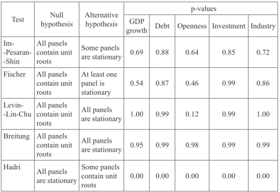
Following the PMG procedure, statistical properties of the variables of interest need to be tested, so, the first step of our empirical analysis was to perform panel unit root tests. According to literature (Breitung and Pesaran, 2005; Moon and Perron, 2004; Pesaran, 2005), panel-based unit root tests have higher power than unit root test based on individual time series. In our analysis we use a battery of unit root tests, namely tests with common unit root processes: LLC (Levin et al., 2002), Breitung (Breitung, 2001), and Hadri (Hadri, 2000) as well as tests with individual unit root processes: IPS (Im et al., 2003) and Fisher ADF test (Maddala and Wu, 1999; Choi, 2001). Table 1 summarizes panel unit root test results.
Table 1: Panel unit root tests results Test hypothesisNull Alternative hypothesis
p-values GDP
growth Debt Openness Investment Industry Im- -Pesaran- -Shin All panels contain unit roots Some panels are stationary 0.69 0.88 0.64 0.85 0.72
Fischer All panels contain unit roots At least one panel is stationary 0.54 0.87 0.46 0.99 0.86 Levin-
-Lin-Chu All panels contain unit roots
All panels
are stationary 1.00 0.99 0.12 0.99 1.00
Breitung All panels contain unit roots
All panels
are stationary 0.95 0.99 0.98 0.99 0.99
Hadri All panels are stationary
Some panels contain unit
roots 0.00 0.00 0.00 0.00 0.00
Note: Levin-Lin-Chu, Breitung and Hadri tests require a balanced panel and were therefore applied to a truncated version of the dataset. Automatic lag length selection is based on Schwarz Criterion and Barlett Kernel. All tests include constant and trend.
According to the results of panel unit root tests, for all series of interest, the null hypothesis of a unit root cannot be rejected. In the case of Hadri test, we strongly reject the null of stationarity. Since, we confirmed that the series are non-stationary, we proceed with panel cointegration tests.
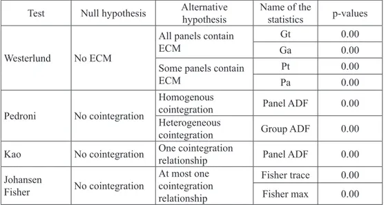
There are several ways of testing the null hypothesis of no cointegration and such tests can be grouped in two large families: the residual-based ones (Pedroni, 1999; Pedroni, 2004; Kao, 1999), constructed on the basis of the Engle and Granger`s (1987) test and likelihood-based ones (Maddala and Wu, 1999) which represent the generalization of Johansen (1991, 1996) test for vector auto-regressive models to panel data. Additionally, we use four new panel cointegration tests developed by Westerlund (2007) which are based on structural dynamic, where the main idea is to test the null hypothesis of no cointegration by inferring whether the error-correction term in a conditional panel error-error-correction model is equal to zero. Table 2 summarizes the panel cointegration test results.
Table 2: Panel cointegration tests results: GDP growth and debt
Test Null hypothesis Alternativehypothesis Name of the statistics p-values
Westerlund No ECM
All panels contain ECM
Gt 0.00
Ga 0.00
Some panels contain
ECM PaPt 0.000.00
Pedroni No cointegration
Homogenous
cointegration Panel ADF 0.00
Heterogeneous
cointegration Group ADF 0.00
Kao No cointegration One cointegration relationship Panel ADF 0.00 Johansen Fisher No cointegration At most one cointegration relationship Fisher trace 0.00 Fisher max 0.00
Note: All tests include constant and trend. Source: Authors’ calculations
According to the results presented in Table 2, the null hypothesis of no cointegration (or no error correction in case of Westerlund tests) is strongly rejected for the variables of interest, so we can estimate the model given in equation (3) which will provide reliable inference about the long-run and short-run influence of general government gross debt, trade openness, total investment and industry value added on GDP growth.
5. Results analysis and discussion
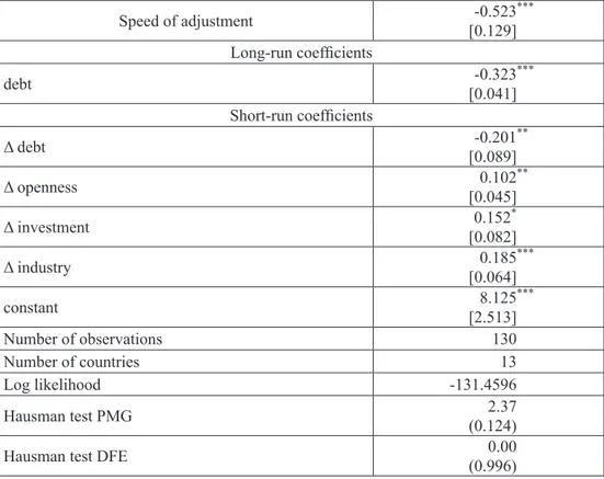
The Table 3 presents the results of the baseline model of GDP growth specified by the equation (3). Furthermore, the Hausman test of long-run homogeneity of coefficients is employed in order to determine which estimator is more appropriate. According to Pesaran et al. (1999), the MG estimator provides consistent estimates of the mean of long-run coefficients, but these are inefficient if slope homogeneity assumption holds. However, if the slope coefficients are indeed homogeneous, than PMG estimator is consistent and efficient. According to Table 3, homogeneity restriction is not rejected by the data, implying that the PMG estimator is efficient under the null hypothesis and is preferred over the MG estimator.
Table 3: Pooled mean group estimates for panel of 14 European countries
Speed of adjustment [0.129]-0.523*** Long-run coefficients debt [0.041]-0.323*** Short-run coefficients Δ debt [0.089]-0.201** Δ openness [0.045]0.102** Δ investment [0.082]0.152* Δ industry [0.064]0.185*** constant [2.513]8.125*** Number of observations 130 Number of countries 13 Log likelihood -131.4596 Hausman test PMG (0.124)2.37
Hausman test DFE (0.996)0.00
Note: Estimations are performed using the PMG estimator of Pesaran et al. (1999); the reported short-run coefficients and the speed of adjustment are simple averages of country-specific coefficients; all equations include a constant term; standard errors are in brackets, p values are in parenthesis; ***, **, * denote significance at 1, 5 and 10 percent confidence level,
respectively. Hausman test PMG denotes test for long-run homogeneity. Hausman test DFE denotes endogeneity test.
The lower part of Table 3 presents Hausman type tests of long-run homogeneity restriction as well as test of endogeneity bias. Namely, homogeneity of long-run coefficients implied by PMG estimating procedure cannot be assumed a priori but needs to be tested. In a manner of Pesaran et al. (1999) we compared two estimators: MG and PMG. When long-run homogeneity restriction is true, PMG estimates would be more efficient compared to MG, but if the true model is heterogeneous, then PMG estimates would be inconsistent. According to test results, we cannot reject the null of long-run homogeneity restriction, so the PMG estimator is appropriate in our case, also simultaneous equation bias from the endogeneity between the error term and the lagged dependent variable is minimal. According to results presented in Table 3, error correction mechanism is in place, since the adjustment coefficient has the correct negative sign and is statistically significant on 1% significance level. The average value of the error correction coefficient (according to PMG estimator) is -0.523 implying that equilibrium is reached in less than 2 years. Furthermore, in the long-run, debt significantly influences the GDP growth having a negative sign as expected and pointing out that government gross debt lowers the GDP growth. In the short run, debt has statistically significant negative influence on GDP growth, as well, with somewhat smaller coefficient when compared to the long run. Furthermore, according to estimated model, all three control variables have statistically significant influence on GDP growth in the short run, with economically meaningful signs, stressing a positive influence of those variables on GDP growth, with industry having the largest coefficient (0.185).
6. Concluding remarks
The empirical results suggest negative relationship between public debt and economic growth controlling for other determinants of growth (trade openness, industry value added and total investment). This inverse debt-growth relationship is in line with previous empirical research and confirms the research hypothesis. We find that the effects of global economic and financial crisis contributed to our empirical results. Prior to crisis, most of CESEE countries experienced stable or declining levels of public debt as fiscal deficits were compensated by higher growth rates. When the crisis emerged, the sharp fall in output was followed by an increase in government expenditures and a decrease in government revenues leading to rising public deficit. The concerns about public debt sustainability widened sovereign spreads and stressed the need to reconsider fiscal policy actions. CESEE countries were faced with a difficult task – most of them implemented fiscal consolidation while the private sector performance created the need for further fiscal stimulus. According to the empirical results and the negative impact of increase in public debt on economic activity, we find that
the fiscal consolidation should be continued combined with policies to promote lasting growth in order to reach debt-stabilizing levels. We find that designing policy frameworks that encourage export, promote industrial development and create better environment for long-term investment foster sustainable growth. The policy mix chosen to reduce the underlying government deficits and prevent further debt accumulation may vary depending on country-specific economic and fiscal policies. The heterogeneity in output effects of fiscal adjustment based on spending cuts, tax increases or other measures aimed at reducing fiscal deficit are beyond the scope of this paper.
The main limitations of our research are short time series. Namely, since the database for the CESEE countries are not available for all governments before 2000, our study was conducted for the period of 12 years. Furthermore, the pooled mean group estimator which assumes homogeneous long-run coefficients has a practical advantage that the short-run dynamics can be determined by available data for each country, taking into account the number of time-series observations in each case by choosing appropriate leg length. Moreover, important issue is the interpretation of heterogeneity which raises obvious problems for inference and requires further analysis. Further research should also include public capital formation in order to explore whether government borrowed funds to finance current spending or to increase public capital.
References
Baum, A., Checherita-Westphal, C., Rother, P. (2013) “Debt and growth: new evidence for the Euro area”, Journal of International Money and Finance, 32, pp. 809-821.
Breitung, J. (2001) “The local power of some unit root tests for panel data”,
Advances in Econometrics, 15, pp. 161-177.
Breitung, J., Pesaran, M. H. (2005) “Unit rots and cointegration in panels”, In L. Matyas and P. Sevestre (eds.) The Econometrics of Panel data: Fundamentals and recent developments in theory and practice, Springer.
Cantor, R., Packer, F. (1996) “Determinants and Impact of Sovereign Credit Ratings”, Federal Reserve Bank of New York, Economic Policy Review, 2(2), pp. 37-54.
Carnot, N. (2013) “The Composition of Fiscal Adjustments: Some Principles”,
ECFIN Economic Brief, 23 (April).
Choi, I. (2001) “Unit root tests for panel data”, Journal of International Money and Finance, 20(2), pp. 249-272.
Cecchetti, S. G., Mohanty, M. S., Zampolli, F. (2011) “The real effects of debt”, BIS Working Paper 352, Bank for International Settlements.
Checherita, C., Rother, P. (2010) “The impact of high and growing government debt on economic growth: en empirical investigation for the euro area”, Working Paper Series 1237, European Central Bank.
Cordella, T., Ricci, L. A., Ruiz-Arranz, M. (2010) “Debt Overhang or Debt Irrelevance?”, IMF Staff Papers 57(1), International Monetary Fund.
Engle, R., Granger, C. (1987) “Cointegration and error correction: representation, estimation, and testing”, Econometrica, 55(2), pp. 251-276.
Hadri, K. (2000) “Testing for stationarity in heterogeneous panel data”, Econometrics Journal, 3(2), pp. 148-161.
Hellwig, M., Neumann, M. J. M. (1987) “Economic policy in Germany: Was there a turnaround? ”, Economic Policy, 5 (October), pp. 105-40.
Hoogduin, L., Öztürk, B., Wierts, P. (2010) “Public Debt Managers’ Behaviour: Interaction with Macro Policies”, DNB Working Paper 273.
Im, K. S., Pesaran, M., Shin, Y. (2003) “Testing for unit roots in heterogeneous panels”, Journal of Econometrics, 115(1), pp. 53-74.
Imbs, J., Rancire, R. (2005) “The overhang hangover”, Economics Working Papers
878, Department of Economics and Business, Universitat Pompeu Fabra. International Monetary Fund (2008) World Economic Outlook October 2008:
Financial Stress, Downturns, and Recoveries. World Economic and Financial Surveys, Washington, D.C.: International Monetary Fund.
International Monetary Fund (2011) “Managing Sovereign Debt and Debt Markets through a Crisis—Practical Insights and Policy Lessons”, Monetary and Capital Markets Department, Downloaded from: http://www.imf.org/external/np/pp/ eng/2011/041811.pdf (01.06.2013.).
Johansen, S. (1991) “Estimation and hypothesis testing of cointegration vectors in Gaussian vector autoregressive models”, Econometrica, 59(6), pp. 1551-1580. Johansen, S. (1996) Likelihood Based Inference on Cointegration in the Vector
Autoregressive Model, (2nd ed.), USA: Oxford University Press.
Kao, C. (1999) “Spurious regression and residual-based tests for cointegration in panel data”, Journal of Econometrics, 90, pp. 1-44.
Keiko, H. (2007) “The Golden Rule and the Economic Cycles”, IMF Working Paper, 199.
Kumar, M. S., Woo, J. (2010) “Public Debt and Growth”, IMF Working Paper, 174. Levin, A., Lin, C.-F., Chu, C.-S. J. (2002) “Unit root test in panel data: asymptotic
and finite sample properties”, Journal of Econometrics, 108, pp. 1-24.
Maddala, G. S., Wu, S. (1999) “A comparative study of unit root tests with panel data and a new simple test”, Oxford Bulletin of Economics and Statistics, 61(S1), pp. 631-652.
Moon, H. R., Perron, B. (2004) “Testing for unit root in panels with dynamic factors”, Journal of Econometrics 122, pp. 81-126.
OECD (2010) “Choosing a Broad Base – Low Rate Approach to Taxation”, OECD Tax Policy Studies, 19, OECD Publishing.
Pattillo, C., Poirson, H., Ricci, L. A. (2011) “External Debt and Growth”, Review of Economics and Institutions, 2(3), pp. 1-30.
Pedroni, P. (1999) “Critical values for cointegration tests in heterogeneous panels with multiple regressors”, Oxford Bulletin of Economics and Statistics, 61(S1), pp. 653-678.
Pedroni, P. (2004) “Panel cointegration: asymptotic and finite sample properties of pooled time series tests with an application to the PPP hypothesis”, Econometric Theory, 20(3), pp. 597-625.
Pesaran, M. H. (2005). Estimation and inference in large heterogeneous panels with a multifactor error structure, Econometrica 74, pp. 967-1012.
Pesaran, M. H., Shin, Y., Smith, R. P. (1999) “Pooled Mean Group Estimation of Dynamic Heterogeneous Panels”, Journal of the American Statistical Association, 94(446), pp. 621-634.
Reinhart, C. M., Rogoff, K. S. (2009) “The Aftermath of Financial Crisis”, NBER
Working Paper Series 14656.
Reinhart, C. M., Reinhart, V. R., Rogoff, K. S. (2012) “Debt Overhangs: Past and Present”, NBER Working Paper Series 18015.
Sándor, G., Martin, R. (2010) “The Impact of the Global Economic and Financial Crisis on Central, Eastern and South-Eastern Europe: A Stock-Taking Exercise”,
Occasional Paper Series 114, European Central Bank.
Schclarek, A. (2004) “Debt and Economic Growth in Developing and Industrial Countries”, Working Papers 34, Lund University: Department of Economics. Westerlund, J. (2007) “Testing for error correction in panel data”, Oxford Bulletin
of Economics and Statistics, 69(6), pp. 709-748.
Woodford, M. (1990) “Public debt as private liquidity”, American Economic Review, 80(2), pp. 382-388.
Odnos javnog duga i ekonomskog rasta: primjer zemalja srednje, istočne i
jugoistočne Europe
Anita Čeh Časni1, Ana Andabaka Badurina2, Martina Basarac Sertić3
Sažetak
Cilj ovog rada bio je kvantificirati dugoročan i kratkoročan odnos duga i ekonomske aktivnosti u zemljama srednje, istočne i jugoistočne Europe. Stoga je, kako bi se istražio utjecaj javnog duga na ekonomski rast, primijenjen združeni procjenitelj aritmetičke sredine grupe (PMG) za razdoblje od 2000. do 2011. godine. Prije izvođenja dinamičke panel analize na temelju PMG procjenitelja, provedeni su testovi jediničnog korijena, kao i testovi panel kointegracije. Prema empirijskim rezultatima, javni dug u dugom roku značajno utječe na rast BDP-a, te ima očekivani negativni predznak. Nadalje, u kratkom roku, dug također ima statistički značajan negativan utjecaj na rast BDP-a, uz značajnost ostalih odrednica rasta (trgovinske otvorenosti, ukupnih investicija i dodane vrijednosti industrije). Preporuča se kreiranje mjera za poticanje izvoza i razvoja industrije te stvaranje boljeg okruženja koje pogoduje dugoročnim investicijama kako bi se potaknuo gospodarski rast. Zaključuje se da treba provoditi kredibilnu strategiju fiskalne konsolidacije zajedno s mjerama za poticanje dugoročnog rasta s ciljem stabiliziranja udjela duga u BDP-u.
Ključne riječi: javni dug, ekonomski rast, združeni procjenitelj aritmetičke sredine grupe, europske zemlje
JEL klasifikacija: C33, F43, H63
1 Dr.sc., viši asistent, Sveučilište u Zagrebu, Ekonomski fakultet, Trg J. F. Kennedyja 6, 10000 Zagreb, Hrvatska. Znanstveni interes: poslovna statistika, multivarijatna statistika, primjena ekonometrije u makroekonomiji. Tel.: +385 1 2383 353. E-mail: aceh@efzg.hr. Osobna web stranica: http://www.efzg.unizg.hr/aceh.
2 Dr.sc., viši asistent, Sveučilište u Zagrebu, Ekonomski fakultet, Trg J. F. Kennedyja 6, 10000 Zagreb, Hrvatska. Znanstveni interes: makroekonomija, upravljanje javnim dugom. Tel.: +385 1 2383 229. E-mail: aandabaka@efzg.hr. Osobna web stranica: http://www.efzg.unizg.hr/ default.aspx?id=2771.
3 Dr.sc., viši asistent, Hrvatska akademija znanosti i umjetnosti, Strossmayerov trg 2, 10000 Zagreb, Hrvatska. Znanstveni interes: ekonomski razvoj, makroekonomski pokretači rasta, konkurentnost industrije, dinamička analiza. Tel.: +385 1 4895 105. E-mail: mbasarac@hazu.hr.
Appendix
Table 1: List of variables
Variable Description Measure Source
GDP_growth Annual percentage growth rate In percentage World Bank
Debt General government gross debt Percent of GDP IMF WEO
Openness Trade openness Percent of GDP World Bank
Investment Ratio of total investment Percent of GDP IMF WEO
Industry Industry, value added annual % growth World Bank
Source: Authors
Table 2: Descriptive statistics of variables used in the empirical analysis (Stata 12) Variable observationsNumber of Mean deviationStandard Minimum Maximum
GDP_growth 204 3.468742 4.261414 -17.95499 12.23323 Debt 200 38.84293 24.50772 3.685 241.653 Openness 203 108.0728 30.11019 56.62534 179.0752 Investment 191 24.73242 5.56825 8.154 40.671 Industry 191 4.179716 8.306424 -26.84759 35.66742 Source: Authors