Building Probabilistic Graphical
Models with Python
Solve machine learning problems using probabilistic
graphical models implemented in Python with
real-world applications
Kiran R Karkera
Copyright © 2014 Packt Publishing
All rights reserved. No part of this book may be reproduced, stored in a retrieval system, or transmitted in any form or by any means, without the prior written permission of the publisher, except in the case of brief quotations embedded in critical articles or reviews.
Every effort has been made in the preparation of this book to ensure the accuracy of the information presented. However, the information contained in this book is sold without warranty, either express or implied. Neither the author, nor Packt Publishing, and its dealers and distributors will be held liable for any damages caused or alleged to be caused directly or indirectly by this book.
Packt Publishing has endeavored to provide trademark information about all of the companies and products mentioned in this book by the appropriate use of capitals. However, Packt Publishing cannot guarantee the accuracy of this information.
First published: June 2014
Production reference: 1190614
Published by Packt Publishing Ltd. Livery Place
35 Livery Street
Birmingham B3 2PB, UK. ISBN 978-1-78328-900-4 www.packtpub.com
Credits
Author
Kiran R Karkera
Reviewers Mohit Goenka Shangpu Jiang Jing (Dave) Tian Xiao Xiao
Commissioning Editor Kartikey Pandey
Acquisition Editor Nikhil Chinnari
Content Development Editor Madhuja Chaudhari
Technical Editor Krishnaveni Haridas
Copy Editors Alisha Aranha Roshni Banerjee Mradula Hegde
Project Coordinator Melita Lobo
Proofreaders Maria Gould Joanna McMahon
Indexers
Mariammal Chettiyar Hemangini Bari
Graphics Disha Haria Yuvraj Mannari Abhinash Sahu
Production Coordinator Alwin Roy
About the Author
Kiran R Karkera
is a telecom engineer with a keen interest in machine learning. He has been programming professionally in Python, Java, and Clojure for more than 10 years. In his free time, he can be found attempting machine learning competitions at Kaggle and playing the flute.About the Reviewers
Mohit Goenka
graduated from the University of Southern California (USC) with a Master's degree in Computer Science. His thesis focused on game theory and human behavior concepts as applied in real-world security games. He also received an award for academic excellence from the Office of International Services at the University of Southern California. He has showcased his presence in various realms of computers including artificial intelligence, machine learning, path planning, multiagent systems, neural networks, computer vision, computer networks, and operating systems.During his tenure as a student, Mohit won multiple competitions cracking codes and presented his work on Detection of Untouched UFOs to a wide range of audience. Not only is he a software developer by profession, but coding is also his hobby. He spends most of his free time learning about new technology and grooming his skills. What adds a feather to Mohit's cap is his poetic skills. Some of his works are part of the University of Southern California libraries archived under the cover of the Lewis Carroll Collection. In addition to this, he has made significant contributions by volunteering to serve the community.
Science at the University of Oregon. He is a member of the OSIRIS lab. His research direction involves system security, embedded system security, trusted computing, and static analysis for security and virtualization. He is interested in Linux kernel hacking and compilers. He also spent a year on AI and machine learning direction and taught the classes Intro to Problem Solving using Python and Operating Systems in the Computer Science department. Before that, he worked as a software developer in the Linux Control Platform (LCP) group at the Alcatel-Lucent (former Lucent Technologies) R&D department for around four years. He got his Bachelor's and Master's degrees from EE in China.
Thanks to the author of this book who has done a good job for both Python and PGM; thanks to the editors of this book, who have made this book perfect and given me the opportunity to review such a nice book.
www.PacktPub.com
Support files, eBooks, discount offers and more
You might want to visit www.PacktPub.com for support files and downloads related to your book.Did you know that Packt offers eBook versions of every book published, with PDF and ePub files available? You can upgrade to the eBook version at www.PacktPub. com and as a print book customer, you are entitled to a discount on the eBook copy. Get in touch with us at [email protected] for more details.
At www.PacktPub.com, you can also read a collection of free technical articles, sign up for a range of free newsletters and receive exclusive discounts and offers on Packt books and eBooks.
TM
http://PacktLib.PacktPub.com
Do you need instant solutions to your IT questions? PacktLib is Packt's online digital book library. Here, you can access, read and search across Packt's entire library of books.
Why Subscribe?
• Fully searchable across every book published by Packt • Copy and paste, print and bookmark content
• On demand and accessible via web browser
Free Access for Packt account holders
Table of Contents
Preface 1
Chapter 1: Probability
5
The theory of probability 5
Goals of probabilistic inference 8
Conditional probability 9
The chain rule 9
The Bayes rule 9
Interpretations of probability 11
Random variables 13
Marginal distribution 13
Joint distribution 14
Independence 14
Conditional independence 15
Types of queries 16
Probability queries 16
MAP queries 16
Summary 18
Chapter 2: Directed Graphical Models
19
Graph terminology 19
Python digression 20
Independence and independent parameters 20
The Bayes network 23
The chain rule 24
Reasoning patterns 24
Causal reasoning 25
Evidential reasoning 27
D-separation 29
The D-separation example 31 Blocking and unblocking a V-structure 33
Factorization and I-maps 34
The Naive Bayes model 34
The Naive Bayes example 36
Summary 37
Chapter 3: Undirected Graphical Models
39
Pairwise Markov networks 39
The Gibbs distribution 41
An induced Markov network 43
Factorization 43
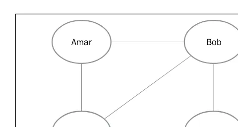
Flow of influence 44
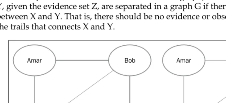
Active trail and separation 45
Structured prediction 45
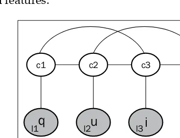
Problem of correlated features 46
The CRF representation 46
The CRF example 47
The factorization-independence tango 48
Summary 49
Chapter 4: Structure Learning
51
The structure learning landscape 52
Constraint-based structure learning 52
Part I 52
Part II 53
Part III 54
Summary of constraint-based approaches 60
Score-based learning 60
The likelihood score 61
The Bayesian information criterion score 62
The Bayesian score 63
Summary of score-based learning 68
Summary 68
Chapter 5: Parameter Learning
69
The likelihood function 71
Parameter learning example using MLE 72
MLE for Bayesian networks 74
Bayesian parameter learning example using MLE 75
Effects of data fragmentation on parameter estimation 77
Bayesian parameter estimation 79
An example of Bayesian methods for parameter learning 80
Bayesian estimation for the Bayesian network 85
Example of Bayesian estimation 85
Summary 91
Chapter 6: Exact Inference Using Graphical Models
93
Complexity of inference 93
Real-world issues 94
Using the Variable Elimination algorithm 94
Marginalizing factors that are not relevant 97
Factor reduction to filter evidence 98
Shortcomings of the brute-force approach 100
Using the Variable Elimination approach 100
Complexity of Variable Elimination 106
Graph perspective 107
Learning the induced width from the graph structure 109
The tree algorithm 110
The four stages of the junction tree algorithm 111 Using the junction tree algorithm for inference 112
Stage 1.1 – moralization 113
Stage 1.2 – triangulation 114
Stage 1.3 – building the join tree 114
Stage 2 – initializing potentials 115
Stage 3 – message passing 115
Summary 119
Chapter 7: Approximate Inference Methods
121
The optimization perspective 121
Belief propagation in general graphs 122 Creating a cluster graph to run LBP 123
Message passing in LBP 124
Steps in the LBP algorithm 125
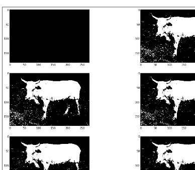
Improving the convergence of LBP 126 Applying LBP to segment an image 126
Understanding energy-based models 128
Visualizing unary and pairwise factors on a 3 x 3 grid 129
Creating a model for image segmentation 130
Applications of LBP 135
Sampling-based methods 136
Forward sampling 136
The Markov Chain Monte Carlo sampling process 138
The Markov property 138
The Markov chain 139
Reaching a steady state 140
Sampling using a Markov chain 140
Gibbs sampling 141
Steps in the Gibbs sampling procedure 141
An example of Gibbs sampling 142
Summary 145
Appendix: References
147
Preface
In this book, we start with an exploratory tour of the basics of graphical models, their types, why they are used, and what kind of problems they solve. We then explore subproblems in the context of graphical models, such as their representation, building them, learning their structure and parameters, and using them to answer our inference queries.
This book attempts to give just enough information on the theory, and then use code samples to peep under the hood to understand how some of the algorithms are implemented. The code sample also provides a handy template to build graphical models and answer our probability queries. Of the many kinds of graphical
models described in the literature, this book primarily focuses on discrete Bayesian networks, with occasional examples from Markov networks.
What this book covers
Chapter 1, Probability, covers the concepts of probability required to understand the graphical models.
Chapter 2, Directed Graphical Models, provides information about Bayesian networks, their properties related to independence, conditional independence, and D-separation. This chapter uses code snippets to load a Bayes network and understand its independence properties.
Chapter 3, Undirected Graphical Models, covers the properties of Markov networks, how they are different from Bayesian networks, and their independence properties.
Chapter 5, Parameter Learning, covers the maximum likelihood and Bayesian approaches to parameter learning with code samples from PyMC.
Chapter 6, Exact Inference Using Graphical Models, explains the Variable Elimination algorithm for accurate inference and explores code snippets that answer our inference queries using the same algorithm.
Chapter 7, Approximate Inference Methods, explores the approximate inference for networks that are too large to run exact inferences on. We will also go through the code samples that run approximate inferences using loopy belief propagation on Markov networks.
Appendix, References, includes all the links and URLs that will help to easily understand the chapters in the book.
What you need for this book
To run the code samples in the book, you'll need a laptop or desktop with IPython installed. We use several software packages in this book, most of them can be installed using the Python installation procedure such as pip or easy_install. In some cases, the software needs to be compiled from the source and may require a C++ compiler.
Who this book is for
This book is aimed at developers conversant with Python and who wish to explore the nuances of graphical models using code samples.
This book is also ideal for students who have been theoretically introduced to graphical models and wish to realize the implementations of graphical models and get a feel for the capabilities of different (graphical model) libraries to deal with real-world models.
Machine-learning practitioners familiar with classification and regression models and who wish to explore and experiment with the types of problems graphical models can solve will also find this book an invaluable resource.
Conventions
In this book, you will find a number of styles of text that distinguish between different kinds of information. Here are some examples of these styles, and an explanation of their meaning.
Code words in text, database table names, folder names, filenames, file extensions, pathnames, dummy URLs, user input, and Twitter handles are shown as follows: "We can do the same by creating a TfidfVectorizer object."
A block of code is set as follows: clf = MultinomialNB(alpha=.01)
print "CrossValidation Score: ", np.mean(cross_validation.cross_val_ score(clf,vectors, newsgroups.target, scoring='f1'))
CrossValidation Score: 0.954618416381
Warnings or important notes appear in a box like this.
Tips and tricks appear like this.
Reader feedback
Feedback from our readers is always welcome. Let us know what you think about this book—what you liked or may have disliked. Reader feedback is important for us to develop titles that you really get the most out of.
To send us general feedback, simply send an e-mail to [email protected], and mention the book title via the subject of your message.
If there is a topic that you have expertise in and you are interested in either writing or contributing to a book, see our author guide on www.packtpub.com/authors.
Customer support
Downloading the example code
You can download the example code files for all Packt books you have purchased from your account at http://www.packtpub.com. If you purchased this book elsewhere, you can visit http://www.packtpub.com/support and register to have the files e-mailed directly to you.
Errata
Although we have taken every care to ensure the accuracy of our content, mistakes do happen. If you find a mistake in one of our books—maybe a mistake in the text or the code—we would be grateful if you would report this to us. By doing so, you can save other readers from frustration and help us improve subsequent versions of this book. If you find any errata, please report them by visiting http://www.packtpub. com/submit-errata, selecting your book, clicking on the erratasubmissionform link, and entering the details of your errata. Once your errata are verified, your submission will be accepted and the errata will be uploaded on our website, or added to any list of existing errata, under the Errata section of that title. Any existing errata can be viewed by selecting your title from http://www.packtpub.com/support.
Piracy
Piracy of copyright material on the Internet is an ongoing problem across all media. At Packt, we take the protection of our copyright and licenses very seriously. If you come across any illegal copies of our works, in any form, on the Internet, please provide us with the location address or website name immediately so that we can pursue a remedy.
Please contact us at [email protected] with a link to the suspected pirated material.
We appreciate your help in protecting our authors, and our ability to bring you valuable content.
Questions
Probability
Before we embark on the journey through the land of graphical models, we must equip ourselves with some tools that will aid our understanding. We will first start with a tour of probability and its concepts such as random variables and the types of distributions.
We will then try to understand the types of questions that probability can help us answer and the multiple interpretations of probability. Finally, we will take a quick look at the Bayes rule, which helps us understand the relationships between probabilities, and also look at the accompanying concepts of conditional probabilities and the chain rule.
The theory of probability
We often encounter situations where we have to exercise our subjective belief about an event's occurrence; for example, events such as weather or traffic that
are inherently stochastic. Probability can also be understood as the degree of subjective belief.
The axioms of probability that have been formulated by Kolmogorov are stated as follows:
• The probability of an event is a non-negative real number (that is, the
probability that it will rain today may be small, but nevertheless will be greater than or equal to 0). This is explained in mathematical terms as follows:
(E)
, (E) 0
P
P
E
F where F is the event space
• The probability of the occurrence of some event in the sample space is 1 (that is, if the weather events in our sample space are rainy, sunny, and cloudy, then one of these events has to occur), as shown in the following formula:
( ) 1
P
Ω =
where
Ω
is the sample space
• The sum of the probabilities of mutually exclusive events gives their union, as given in the following formula:
(
1 2)
( )
When we discuss about the fairness (or unfairness) of a dice or a coin flip, we are discussing another key aspect of probability, that is, model parameters. The idea of a fair coin translates to the fact that the controlling parameter has a value of 0.5 in favor of heads, which also translates to the fact that we assume all the outcomes to be equally likely. Later in the book, we shall examine how many parameters are required to completely specify a probability distribution. However, we are getting ahead of ourselves. First let's learn about probability distribution.
A probability distribution consists of the probabilities associated with each
measurable outcome. In the case of a discrete outcome (such as a throw of a dice or a coin flip), the distribution is specified by a probability mass function, and in the case of a continuous outcome (such as the height of students in a class), it is specified by a probability density function.
A distribution that assigns equal probabilities to all outcomes is called a uniform distribution. This is one of the many distributions that we will explore.
Let's look at one of the common distributions associated with continuous outcomes, that is, the Gaussian or normal distribution, which is in the shape of a bell and hence called a bell curve (though there are other distributions whose shapes are similar to the bell shape). The following are some examples from the real world:
• Heights of students in a class are log-normally distributed (if we take the logarithm of the heights of students and plot it, the resulting distribution is normally distributed)
• Measurement errors in physical experiments
The following graph shows multiple Gaussian distributions with different values of mean and variance. It can be seen that the more variance there is, the broader the distribution, whereas the value of the mean shifts the peak on the x axis, as shown in the following graph:
Goals of probabilistic inference
Now that we have understood the concept of probability, we must ask ourselves how this is used. The kind of questions that we ask fall into the following categories:
• The first question is parameter estimation, such as, is a coin biased or fair? And if biased, what is the value of the parameter?
• The second question is that given the parameters, what is the probability of the data? For example, what is the probability of five heads in a row if we flip a coin where the bias (or parameter) is known.
The preceding questions depend on the data (or lack of it). If we have a set of observations of a coin flip, we can estimate the controlling parameter (that is, parameter estimation). If we have an estimate of the parameter, we would like to estimate the probability of the data generated by the coin flips (the second question). Then, there are times when we go back and forth to improve the model.
Conditional probability
Let us use a concrete example, where we have a population of candidates who are applying for a job. One event (x) could be a set of all candidates who get an offer, whereas another event (y) could be the set of all highly experienced candidates. We might want to reason about the set of a conjoint event (x∩y), which is the set of
experienced candidates who got an offer (the probability of a conjoint event P(x∩y)
is also written as P(x y, )). The question that raises is that if we know that one event has occurred, does it change the probability of occurrence of the other event. In this case, if we know for sure that a candidate got an offer, what does it tell us about their experience?
Conditional probability is formally defined as P( | ) (( ))
p x y possible outcomes of the joint distribution with the value of x summed out, that is,
∑
xP(x, y)=P(y).The chain rule
The chain rule allows us to calculate the joint distribution of a set of random variables using their conditional probabilities. In other words, the joint distribution is the product of individual conditional probabilities. Since P x( ∩y)=P x P y x( ) ( | ), and if
We shall return to this in detail in graphical models, where the chain rule helps us decompose a big problem (computing the joint distribution) by splitting it into smaller problems (conditional probabilities).
The Bayes rule
The Bayes rule is one of the foundations of the probability theory, and we won't go into much detail here. It follows from the definition of conditional probability, as shown in the following formula:
From the formula, we can infer the following about the Bayes rule—we entertain prior beliefs about the problem we are reasoning about. This is simply called the prior term. When we start to see the data, our beliefs change, which gives rise to our final belief (called the posterior), as shown in the following formula:
posterior
α
prior
×
likelihood
Let us see the intuition behind the Bayes rule with an example. Amy and Carl are standing at a railway station waiting for a train. Amy has been catching the same train everyday for the past year, and it is Carl's first day at the station. What would be their prior beliefs about the train being on time?
Amy has been catching the train daily for the past year, and she has always seen the train arrive within two minutes of the scheduled departure time. Therefore, her strong belief is that the train will be at most two minutes late. Since it is Carl's first day, he has no idea about the train's punctuality. However, Carl has been traveling the world in the past year, and has been in places where trains are not known to be punctual. Therefore, he has a weak belief that the train could be even 30 minutes late. On day one, the train arrives 5 minutes late. The effect this observation has on both Amy and Carl is different. Since Amy has a strong prior, her beliefs are modified a little bit to accept that the train can be as late as 5 minutes. Carl's beliefs now change in the direction that the trains here are rather punctual.
In other words, the posterior beliefs are influenced in multiple ways: when
someone with a strong prior sees a few observations, their posterior belief does not change much as compared to their prior. On the other hand, when someone with a weak prior sees numerous observations (a strong likelihood), their posterior belief changes a lot and is influenced largely by the observations (likelihood) rather than their prior belief.
Let's look at a numerical example of the Bayes rule. D is the event that an
athlete uses performance-enhancing drugs (PEDs). T is the event that the drug test returns positive. Throughout the discussion, we use the prime (') symbol to notate that the event didn't occur; for example, D' represents the event that the athlete didn't use PEDs.
The lab doing the drug test claims that it can detect PEDs 90 percent of the time. We also learn that the false-positive rate (athletes whose tests are positive but did not use PEDs) is 15 percent, and that 10 percent of athletes use PEDs. What is the probability that an athlete uses PEDs if the drug test returned positive?
From the basic form of the Bayes rule, we can write the following formula:
( ) ( )
Now, we have the following data: • P(T|D): This is equal to 0.90
• P(T|D'): This is equal to 0.15 (the test that returns positive given that the athlete didn't use PEDs)
• P(D): This is equal to 0.1
When we substitute these values, we get the final value as 0.4, as shown in the following formula:
This result seems a little counterintuitive in the sense that despite testing positive for PEDs, there's only a 40 percent chance that the athlete used PEDs. This is because the use of PEDs itself is quite low (only 10 percent of athletes use PEDs), and that the rate of false positives is relatively high (0.15 percent).
Interpretations of probability
In the previous example, we noted how we have a prior belief and that the
introduction of the observed data can change our beliefs. That viewpoint, however, is one of the multiple interpretations of probability.
The first one (which we have discussed already) is a Bayesian interpretation, which holds that probability is a degree of belief, and that the degree of belief changes before and after accounting for evidence.
To illustrate this with an example, let's go back to the coin flipping experiment, where we wish to learn the bias of the coin. We run two experiments, where we flip the coin 10 times and 10000 times, respectively. In the first experiment, we get 7 heads and in the second experiment, we get 7000 heads.
From a Frequentist viewpoint, in both the experiments, the probability of getting heads is 0.7 (7/10 or 7000/10000). However, we can easily convince ourselves that we have a greater degree of belief in the outcome of the second experiment than that of the first experiment. This is because the first experiment's outcome has a Bayesian perspective that if we had a prior belief, the second experiment's observations would overwhelm the prior, which is unlikely in the first experiment.
For the discussion in the following sections, let us consider an example of a company that is interviewing candidates for a job. Prior to inviting the candidate for an
interview, the candidate is screened based on the amount of experience that the candidate has as well as the GPA score that the candidate received in his graduation results. If the candidate passes the screening, he is called for an interview. Once the candidate has been interviewed, the company may make the candidate a job offer (which is based on the candidate's performance in the interview). The candidate is also evaluating going for a postgraduate degree, and the candidate's admission to a postgraduate degree course of his choice depends on his grades in the bachelor's degree. The following diagram is a visual representation of our understanding of the relationships between the factors that affect the job selection (and postgraduate degree admission) criteria:
Job Offer
Degree score
Job Interview Experience
Random variables
The classical notion of a random variable is the one whose value is subject to
variations due to chance (Wikipedia). Most programmers have encountered random numbers from standard libraries in programming languages. From a programmer's perspective, unlike normal variables, a random variable returns a new value every time its value is read, where the value of the variable could be the result of a new invocation of a random number generator.
We have seen the concept of events earlier, and how we could consider the
probability of a single event occurring out of the set of measurable events. It may be suitable, however, to consider the attributes of an outcome.
In the candidate's job search example, one of the attributes of a candidate is his experience. This attribute can take multiple values such as highly relevant or not relevant. The formal machinery for discussing attributes and their values in different outcomes is called random variables [Koller et al, 2.1.3.1].
Random variables can take on categorical values (such as {Heads, Tails} for the outcomes of a coin flip) or real values (such as the heights of students in a class).
Marginal distribution
We have seen that the job hunt example (described in the previous diagram) has five random variables. They are grades, experience, interview, offer, and admission. These random variables have a corresponding set of events.
Now, let us consider a subset X of random variables, where X contains only the
Experience random variable. This subset contains the events highly relevant and
not relevant.
If we were to enlist the probabilities of all the events in the subset X, it would be called a marginal distribution, an example of which can be found in the following formula:
(
)
0.4,(
)
0.6P Experience=′Highly relevant′ = P Experience=′Not Relevant =
Like all valid distributions, the probabilities should sum up to 1.
Joint distribution
We have seen that the marginal distribution is a distribution that describes a subset of random variables. Next, we will discuss a distribution that describes all the random variables in the set. This is called a joint distribution. Let us look at the joint distribution that involves the Degree score and Experience random variables in the job hunt example:
Degree score
Relevant Experience
Highly relevant
Not relevant
Poor 0.1 0.1 0.2 Average 0.1 0.4 0.5 Excellent 0.2 0.1 0.3
0.4 0.6 1
The values within the dark gray-colored cells are of the joint distribution, and the values in the light gray-colored cells are of the marginal distribution (sometimes called that because they are written on the margins). It can be observed that the individual marginal distributions sum up to 1, just like a normal probability distribution. Once the joint distribution is described, the marginal distribution can be found by summing up individual rows or columns. In the preceding table, if we sum up the columns, the first column gives us the probability for Highly relevant, and the second column for Not relevant. It can be seen that a similar tactic applied on the rows gives us the probabilities for degree scores.
Independence
The concept of independent events can be understood by looking at an example. Suppose we have two dice, and when we roll them together, we get a score of 2 on one die and a score of 3 on the other. It is not difficult to see that the two events are independent of each other because the outcome of a roll of each dice does not influence or interact with the other one.
We can define the concept of independence in multiple ways. Assume that we have two events a and b and the probability of the conjunction of both events is simply the product of their probabilities, as shown in the following formula:
If we were to write the probability of P a b
(
,)
as P a P b( ) ( | a) (that is, the product of probability of a and probability of b given that the event a has happened), if the events a and b are independent, they resolve to P a P b( ) ( ).An alternate way of specifying independence is by saying that the probability of a
given b is simply the probability of a, that is, the occurrence of b does not affect the probability of a, as shown in the following formula:
(
)
(
|)
( )
( )
0P= a⊥b if P a b =P a or if P b =
It can be seen that the independence is symmetric, that is,
(
a⊥b implies b)
(
⊥a)
. Although this definition of independence is in the context of events, the same concept can be generalized to the independence of random variables.Conditional independence
Given two events, it is not always obvious to determine whether they are
independent or not. Consider a job applicant who applied for a job at two companies, Facebook and Google. It could result in two events, the first being that a candidate gets an interview call from Google, and another event that he gets an interview call from Facebook. Does knowing the outcome of the first event tell us anything about the probability of the second event? Yes, it does, because we can reason that if a candidate is smart enough to get a call from Google, he is a promising candidate, and that the probability of a call from Facebook is quite high.
What has been established so far is that both events are not independent. Supposing we learn that the companies decide to send an interview invite based on the
candidate's grades, and we learn that the candidate has an A grade, from which we infer that the candidate is fairly intelligent. We can reason that since the candidate is fairly smart, knowing that the candidate got an interview call from Google does not tell us anything more about his perceived intelligence, and that it doesn't change the probability of the interview call from Facebook. This can be formally annotated as the probability of a Facebook interview call, given a Google interview call AND grade A, is equal to the probability of a Facebook interview call given grade A, as shown in the following formula:
(
| ,)
(
|)
Pr Facebook Google GradeA =Pr Facebook GradeA
Types of queries
Having learned about joint and conditional probability distributions, let us turn our attention to the types of queries we can pose to these distributions.
Probability queries
This is the most common type of query, and it consists of the following two parts: • The evidence: This is a subset E of random variables which have
been observed
• The query: This is a subset Y of random variables
We wish to compute the value of the probability P Y E
(
| =e)
, which is the posteriorprobability or the marginal probability over Y. Using the job seeker example again, we can compute the marginal distribution over an interview call, conditioned on the fact that Degree score = Grade A.
MAP queries
Maximum a posteriori (MAP) is the highest probability joint assignment to some subsets of variables. In the case of the probability query, it is the value of the probability that matters. In the case of MAP, calculating the exact probability value of the joint assignment is secondary as compared to the task of finding the joint assignment to all the random variables.
It is possible to return multiple joint assignments if the probability values are equal. We shall see from an example that in the case of the joint assignment, it is possible that the highest probability from each marginal value may not be the highest joint assignment (the following example is from Koller et al).
Consider two non-independent random variables X and Y, where Y is dependent on
X. The following table shows the probability distribution over X:
X0 X1
We can see that the MAP assignment for the random variable X is X1 since it has a higher value. The following table shows the marginal distribution over X and Y:
P(Y|X) Y0 Y1
X0 0.1 0.9 X1 0.5 0.5
The joint distribution over X and Y is listed in the following table:
Assignment Value
X0, Y0 0.04 X0, Y1 0.36 X1, Y0 0.3 X1, Y1 0.3
In the joint distribution shown in the preceding table, the MAP assignment to random variables (X, Y) is (X0, Y1), and that the MAP assignment to X (X1) is not a part of the MAP of the joint assignment. To sum up, the MAP assignment cannot be obtained by simply taking the maximum probability value in the marginal distribution for each random variable.
A different type of MAP query is a marginal MAP query where we only have a subset of the variables that forms the query, as opposed to the joint distribution. In the previous example, a marginal MAP query would be MAP (Y), which is the maximum value of the MAP assignment to the random variable Y, which can be read by looking at the joint distribution and summing out the values of X. From the following table, we can read the maximum value and determine that the MAP (Y) is Y1:
Assignment Value
The data for the marginal query has been obtained from
Querying Joint Probability Distributions by Sargur Srihari.
You can find it at http://www.cedar.buffalo.
edu/~srihari/CSE574/Chap8/Ch8-PGM-Directed/8.1.2-QueryingProbabilityDistributions.pdf.
Summary
Directed Graphical Models
In this chapter, we shall learn about directed graphical models, which are also known as Bayesian networks. We start with the what (the problem we are trying to solve), the how (graph representation), the why (factorization and the equivalence of CPD and graph factorization), and then move on to using the Libpgm Python library to play with a small Bayes net.
Graph terminology
Before we jump into Bayes nets, let's learn some graph terminology. A graph G consists of a set of nodes (also called vertices) V=
{
V V1, 2,KVn}
and another set of edges{
1, 2, n}
E= E E KE . An edge that connects a pair of nodes ,
i j
V V can be of two types: directed (represented by Vi→Vj) and undirected (represented by Vi−Vj). A graph can also be represented as an adjacency matrix, which in the case of an undirected graph, if the position G(i,j) contains 1, indicates an edge between i and j vertices. In the case of a directed graph, a value of 1 or -1 indicates the direction of the edge.
In many cases, we are interested in graphs in which all the edges are either directed or undirected, leading to them being called directed graphs or undirected graphs, respectively.
The parents of a V1 node in a directed graph are the set of nodes that have outgoing edges that terminate at V1.
The children of the V1 node are the set of nodes that have incoming edges which leave V1.
The degree of a node is the number of edges it participates in.
If there exists a path from a node that returns to itself after traversing the other nodes, it is called a cycle or loop.
A Directed Acyclic Graph (DAG) is a graph with no cycles.
A Partially Directed Acyclic Graph (PDAG) is a graph that can contain both directed and undirected edges.
A forest is a set of trees.
Python digression
We will soon start to explore GMs using Python, and this is a good time to review your Python installation. The recommended base Python installation for the examples in this book is IPython, which is available for all platforms. Refer to the IPython website for platform-specific documentation.
We shall also use multiple Python libraries to explore various areas of graphical models. Unless otherwise specified, the usual way to install Python libraries is using pip install <packagename> or easy_install <packagename>.
To use the code in this chapter, please install Libpgm (https://pypi.python.org/ pypi/libpgm) and scipy (http://scipy.org/).
Independence and independent
parameters
One of the key problems that graphical models solve is in defining the joint
distribution. Let's take a look at the job interview example where a candidate with a certain amount of experience and education is looking for a job. The candidate is also applying for admission to a higher education program.
Each row contains a probability for the assignment of the random variables in that row. While different instantiations of the table might have different probability assignments, we will need 24 parameters (one for each row) to encode the
information in the table. However, for calculation purposes, we will need only 23 independent parameters. Why do we remove one? Since the sum of probabilities equals 1, the last parameter can be calculated by subtracting one from the sum of the 23 parameters already found.
Experience Grades Interview Offer Probability
0 0 0 0 0 0.7200
1 0 0 0 1 0.0800
2 0 0 1 0 0.0720
3 0 0 1 1 0.1080
. .
Rows elided
21 1 1 1 1 0.1200
22 1 1 2 0 0.0070
23 1 1 2 1 0.6930
The preceding joint distribution is the output of the printjointdistribution. ipynb IPython Notebook, which prints all permutations of the random variables' experience, grades, interview, and offer, along with their probabilities.
It should be clear on observing the preceding table that acquiring a fully specified joint distribution is difficult due to the following reasons:
• It is too big to store and manipulate from a computational point of view • We'll need large amounts of data for each assignment of the joint distribution
to correctly elicit the probabilities
• The individual probabilities in a large joint distribution become vanishingly small and are no longer meaningful to human comprehension
The joint distribution P over Grades and Admission is (throughout this book, the superscript 0 and 1 indicate low and high scores) as follows:
Grades Admission Probability (S,A)
S0 A0 0.665
S0 A1 0.035
S1 A0 0.06
S1 A1 0.24
When we reason about graduate admissions from the perspective of causality, it is clear that the admission depends on the grades, which can also be represented using the conditional probability as follows:
(
,)
( ) (
| S)
P S A =P S P A
The number of parameters required in the preceding formula is three, one parameter for P S
( )
and two each for(
0)
|
P A S and
(
1)
|
How do we calculate the number of parameters in the Bayes net in the preceding diagram? Let's go through each conditional probability table, one parameter at a time. Experience and Grades take two values, and therefore need one independent parameter each. The Interview table has 12 (3 x 4) parameters. However, each row sums up to 1, and therefore, we need two independent parameters per row. The whole table needs 8 (2 x 4) independent parameters. Similarly, the Offer table has six entries, but only 1 independent parameter per row is required, which makes 3 (1 x 3) independent parameters. Therefore, the total number of parameters is 1 (Experience) + 1 (Grades)+ 12 (Interview) + 3 (Offer) amount to 17, which is a lot lesser than 24 parameters to fully specify the joint distribution. Therefore, the independence assumptions in the Bayesian network helps us avoid specifying the joint distribution.
The Bayes network
A Bayes network is a structure that can be represented as a directed acyclic graph, and the data it contains can be seen from the following two points of view:
• It allows a compact and modular representation of the joint distribution using the chain rule for Bayes network
• It allows the conditional independence assumptions between vertices to be observed
We shall explore the two ideas in the job interview example that we have seen so far (which is a Bayesian network, by the way).
The modular structure of the Bayes network is the set of local probability models that represent the nature of the dependence of each variable on its parents (Koller et al 3.2.1.1). One probability distribution each exists for Experience and Grades, and a conditional probability distribution (CPD) each exists for Interview and Offer. A CPD specifies a distribution over a random variable, given all the combinations of assignments to its parents. Thus, the modular representation for a given Bayes network is the set of CPDs for each random variable.
The chain rule
The chain rule allows us to define the joint distribution as a product of factors. In the job interview example, using the chain rule for probability, we can write the following formula:
(
, , ,
)
( )
(
|
)
(
| ,
)
(
O | , ,
)
P E G I O
=
P E
×
P G E
×
P I E G
×
P
E G I
In the preceding formula, E, G, I, and O stand for Experience, Grades, Interview, and
Offer respectively. However, we can use the conditional independence assumptions encoded by the graph to rewrite the joint distribution as follows:
(
, , ,
)
( )
( )
(
| ,
)
(
O |
)
P E G I O
=
P E
×
P G
×
P I E G
×
P
I
This is an example of the chain rule for Bayesian networks. More generally, we can write it as follows:
(
1,
2,
,
n)
(
i|
G(
i)
)
P X X
K
X
=
∏
i P X
Par
X
Here, is a node in the graph G and ParG are the parents of the node in
the graph G.
Reasoning patterns
In this section, we shall look at different kinds of reasoning used in a Bayes network. We shall use the Libpgm library to create a Bayes network. Libpgm reads the
network information such as nodes, edges, and CPD probabilities associated with each node from a JSON-formatted file with a specific format. This JSON file is read into the NodeData and GraphSkeleton objects to create a discrete Bayesian network (which, as the name suggests, is a Bayes network where the CPDs take discrete values). The TableCPDFactorization object is an object that wraps the discrete Bayesian network and allows us to query the CPDs in the network. The JSON file for this example, job_interview.txt, should be placed in the same folder as the IPython Notebook so that it can be loaded automatically.
Causal reasoning
The first kind of reasoning we shall explore is called causal reasoning. Initially, we observe the prior probability of an event unconditioned by any evidence (for this example, we shall focus on the Offer random variable). We then introduce observations of one of the parent variables. Consistent with our logical reasoning, we note that if one of the parents (equivalent to causes) of an event is observed, then we have stronger beliefs about the child random variable (Offer).
We start by defining a function that reads the JSON data file and creates an object we can use to run probability queries. The following code is from the Bayes net-Causal Reasoning.ipynb IPython Notebook:
from libpgm.graphskeleton import GraphSkeleton jsonpath="job_interview.txt" nd.load(jsonpath)
skel.load(jsonpath) # load bayesian network
bn = DiscreteBayesianNetwork(skel, nd) tablecpd=TableCPDFactorization(bn) return tablecpd
We can now use the specificquery function to run inference queries on the
network we have defined. What is the prior probability of getting a P Offer
(
=1)
Offer? Note that the probability query takes two dictionary arguments: the first one being the query and the second being the evidence set, which is specified by an empty dictionary, as shown in the following code:tcpd=getTableCPD()
tcpd.specificquery(dict(Offer='1'),dict())
The following is the output of the preceding code: 0.432816
It is about 43 percent, and if we now introduce evidence that the candidate has poor grades, how does it change the probability of getting an offer? We will evaluate the value of P Offer
(
=1|Grades=0)
, as shown in the following code:tcpd=getTableCPD()
The following is the output of the preceding code: 0.35148
As expected, it decreases the probability of getting an offer since we reason that students with poor grades are unlikely to get an offer. Adding further evidence that the candidate's experience is low as well, we evaluate
(
1| 0, 0)
P Offer= Grades= Experience= , as shown in the following code: tcpd=getTableCPD()
tcpd.specificquery(dict(Offer='1'),dict(Grades='0',Experience='0'))
The following is the output of the preceding code: 0.2078
As expected, it drops even lower on the additional evidence, from 35 percent to 20 percent.
What we have seen is that the introduction of the observed parent random variable strengthens our beliefs, which leads us to the name causal reasoning.
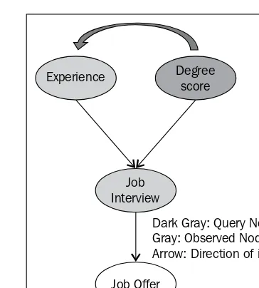
In the following diagram, we can see the different paths taken by causal and evidential reasoning:
Dark Gray: Query Node Gray: Observed Node Arrow: Direction of inference
Evidential Reasoning
Job Offer Job Interview
Experience Degree
score
Causal Reasoning
Job Offer
Degree score
Evidential reasoning
Evidential reasoning is when we observe the value of a child variable, and we wish to reason about how it strengthens our beliefs about its parents. We will evaluate the prior probability of high Experience P Experience
(
=1)
, as shown in the following code:tcpd=getTableCPD()
tcpd.specificquery(dict(Experience='1'),dict())
The output of the preceding code is as follows: 0.4
We now introduce evidence that the candidate's interview was good and evaluate the value for P(Experience=1|Interview=2), as shown in the following code:
tcpd=getTableCPD()
print tcpd.specificquery(dict(Experience='1'),dict(Interview='2'))
The output of the preceding code is as follows: 0.864197530864
We see that if the candidate scores well on the interview, the probability that the candidate was highly experienced increases, which follows the reasoning that the candidate must have good experience or education, or both. In evidential reasoning, we reason from effect to cause.
Inter-causal reasoning
Inter-causal reasoning, as the name suggests, is a type of reasoning where multiple causes of a single effect interact. We first determine the prior probability of having high, relevant experience; thus, we will evaluate P(Experience=1), as shown in the following code:
tcpd=getTableCPD()
tcpd.specificquery(dict(Experience='1'),dict())
By introducing evidence that the interview went extremely well, we think that the candidate must be quite experienced. We will now evaluate the value for
(
1| 2)
P Experience= Interview= , as shown in the following code: tcpd=getTableCPD()
tcpd.specificquery(dict(Experience='1'),dict(Interview='2'))
The following is the output of the preceding code: 0.864197530864
The Bayes network confirms what we think is true (the candidate is experienced), and the probability of high experience goes up from 0.4 to 0.86. Now, if we introduce evidence that the candidate didn't have good grades and still managed to get a good score in the interview, we may conclude that the candidate must be so experienced that his grades didn't matter at all. We will evaluate the value for
(
1| 2, 0)
P Experience= Interview= Grades= , as shown in the following code: tcpd=getTableCPD()
tcpd.specificquery(dict(Experience='1'),dict(Interview='2',Grad es='0'))
The output of the preceding code is as follows: 0.909090909091
This confirms our hunch that even though the probability of high experience went up only a little, it strengthens our belief about the candidate's high experience. This example shows the interplay between the two parents of the Job interview node, which are Experience and Degree Score, and shows us that if we know one of the causes behind an effect, it reduces the importance of the other cause. In other words, we have explained the poor grades on observing the experience of the candidate. This phenomenon is commonly called explaining away.
Dark Gray: Query Node Gray: Observed Node Arrow: Direction of inference
Fig x.x Intercausal Reasoning
Job Offer
Degree score
Job Interview Experience
Bayes networks are usually drawn with the independent events on top and the influence flows from top to bottom (similar to the job interview example). It may be useful to recall causal reasoning flows from top to bottom, evidential reasoning flows from bottom to top, and inter-causal reasoning flows sideways.
D-separation
Having understood that the direction of arrows indicate that one node can influence another node in a Bayes network, let's see how exactly influence flows in a Bayes network. We can see that the grades eventually influence the job offer, but in the case of a very big Bayes network, it would not help to state that the leaf node is influenced by all the nodes at the top of the Bayes network. Are there conditions where influence does not flow? We shall see that there are simple rules that explain the flow of influence in the following table:
No variables observed Y has been observed
X
←
Y
←
Z
JX
←
Y
←
LX
→
Y
→
Z
JX
→
Y
→
Z
LX
←
Y
→
Z
JX
←
Y
→
Z
LThe preceding table depicts the open and closed active trails between three nodes
X, Y, and Z. In the first column, no variables are observed, whereas in the second
column, Y has been observed.
We shall first consider the case where no random variables have been observed. Consider the chains of nodes in the first column of the preceding table. Note that the rules in the first three rows allow the influence to flow from the first to the last node. Influence can flow along the path of the edges, even if these chains are extended for longer sequences. It must be pointed out that the flow of influence is not restricted by the directionality of the links that connect them.
However, there is one case we should watch out for, which is called the V-structure,
X →Y←Z—probably called so because the direction of edges is pointed inwards. In this case, the influence cannot flow from X to Z since it is blocked by Y. In longer chains, the influence will flow unless it is obstructed by a V-structure.
In this case, A→B→X ←Y→Z because of the V-structure at X the influence can flow from A→B→X and X ←Y →Z but not across the node X.
We can now state the concept of an active trail (of influence). A trail is active if it
Let's now look at the second case where we do have observed evidence variables. It is easier to understand if we compare the case with the previous chains, where we observe the random variable Y.
The smiley trails shown in the previous table indicate an active trail, and the others indicate a blocked trail. It can be observed that the introduction of evidence simply negates a previously active trail, and it opens up if a previously blocking V-structure existed.
We can now state that a trail given some evidence will be active if the middle node or any of its descendants in any V-structure (for example, Y or its descendants in X →Y←Z) is present in the evidence set . In other words, observing Y or any of its children will open up the blocking V-structure, making it an active trail. Additionally, as seen in the the following table, an open trail gets blocked by introduction of evidence and vice versa.
Job Offer
Flow of influence with ‘Job Interview’ variable being observed.
We first query the job offer with no other observed variables, as shown in the following code:
getTableCPD().specificquery(dict(Offer='1'),dict())
The output of the preceding code is as follows: 0.432816
We know from the active trail rules that observing Experience should change the probability of the offer, as shown in the following code:
getTableCPD().specificquery(dict(Offer='1'),dict(Experience='1'))
The output of the preceding code is as follows: 0.6438
As per the output, it changes. Now, let's add the Interview observed variable, as shown in the following code:
getTableCPD().specificquery(dict(Offer='1'),dict(Interview='1'))
The output of the preceding code is as follows: 0.6
We get a slightly different probability for Offer. We know from the D-separation rules that observing Interview should block the active trail from Experience to Offer, as shown in the following code:
getTableCPD().specificquery(dict(Offer='1'),dict(Interview='1',Experi ence='1'))
The output of the preceding code is as follows: 0.6
Observe that the probability of Offer does not change from 0.6, despite the addition of the Experience variable being observed. We can add other values of Interview object's parent variables, as shown in the following code:
query=dict(Offer='1')
results=[getTableCPD().specificquery(query,e) for e in [dict(Interview ='1',Experience='0'),
The output of the preceding code is as follows: [0.6, 0.6, 0.6, 0.6]
The preceding code shows that once the Interview variable is observed, the active trail between Experience and Offer is blocked. Therefore, Experience and Offer are conditionally independent when Interview is given, which means observing the values of the interview's parents, Experience and Grades, do not contribute to changing the probability of the offer.
Blocking and unblocking a V-structure
Let's look at the only V-structure in the network, Experience → Interview ← Grades, and see the effect observed evidence has on the active trail.
getTableCPD().specificquery(dict(Grades='1'),dict(Experience='0')) getTableCPD().specificquery(dict(Grades='1'),dict())
The result of the preceding code is as follows: 0.3
0.3
According to the rules of D-separation, the interview node is a V-structure between Experience and Grades, and it blocks the active trails between them. The preceding code shows that the introduction of the observed variable Experience has no effect on the probability of the grades.
getTableCPD().specificquery(dict(Grades='1'),dict(Interview='1'))
The following is the output of the preceding code: 0.413016270338
The following code should activate the trail between Experience and Grades: getTableCPD().specificquery(dict(Grades='1'),dict(Interview='1',Exper ience='0'))
getTableCPD().specificquery(dict(Grades='1'),dict(Interview='1',Exper ience='1'))
The output of the preceding code is as follows: 0.588235294118
0.176470588235
The preceding code now shows the existence of an active trail between Experience and Grades, where changing the observed Experience value changes the
Factorization and I-maps
So far, we have understood that a graph G is a representation of a distribution P. We can formally define the relationship between a graph G and a distribution P in the following way.
If G is a graph over random variables X X1, 2,K,Xn, we can state that a distribution
P factorizes over G if P X X
(
1, 2,K,Xn)
= ∏iP X(
1|ParG(
Xi)
)
. Here, ParG(
Xi)
are the parent nodes of . In other words, a joint distribution can be defined as a product of each random variable when its parents are given.The interplay between factorization and independence is a useful phenomenon that allows us to state that if the distribution factorizes over a graph and given that two nodes X Y Z, | are D-separated, the distribution satisfies those independencies (X Y Z, | ).
Alternately, we can state that the graph G is an Independency map (I-map) for a distribution P, if P factorizes over G because of which we can read the independencies from the graph, regardless of the parameters. An I-map may not encode all the independencies in the distribution. However, if the graph satisfies all the dependencies in the distribution, it is called a Perfect map (P-map). The graph of the job interview is an example of an I-map.
The Naive Bayes model
We can sum this up by saying that a graph can be seen from the following two viewpoints:
• Factorization: This is where a graph allows a distribution to be represented • I-map: This is where the independencies encoded by the graph hold in
the distribution
The Naive Bayes model is the one that makes simplistic independence assumptions. We use the Naive Bayes model to perform binary classification Here, we are given a set of instances, where each instance consists of a set of features X X1, 2,K,Xn and a
class y. The task in classification is to predict the correct class of y when the rest of the features X X1, 2,K,Xn... are given.
For example, we are given a set of newsgroup postings that are drawn from two newsgroups. Given a particular posting, we would like to predict which newsgroup that particular posting was drawn from. Each posting is an instance that consists of a bag of words (we make an assumption that the order of words doesn't matter, just the presence or absence of the words is taken into account), and therefore, the
1, 2, , n
X X K X features indicate the presence or absence of words.
The difference between Naive Bayes and the job candidate example is that Naive Bayes is so called because it makes naïve conditional independence assumptions, and the model factorizes as the product of a prior and individual conditional probabilities, as shown in the following formula:
(
, 1, 2,)
( )
2(
|)
n
n i i
P C X X X P C P X C
=
=
∏
K
Although the term on the left is the joint distribution that needs a huge number of independent parameters (2n+1 - 1 if each feature is a binary value), the Naive Bayes
representation on the right needs only 2n+1 parameters, thus reducing the number of parameters from exponential (in a typical joint distribution) to linear (in Naive Bayes). In the context of the newsgroup example, we have a set of words such as {atheist, medicine, religion, anatomy} drawn from the alt.atheism and sci.med newsgroups. In this model, you could say that the probability of each word appearing is only dependent on the class (that is, the newsgroup) and independent of other words in the posting. Clearly, this is an overly simplified assumption, but it has been shown to have a fairly good performance in domains where the number of features is large and the number of instances is small, such as text classification, which we shall see with a Python program.
Word
n-1 Word n
Class
Word 1 Word 2
The Naive Bayes example
In the Naive Bayes example, we will use the Naive Bayes implementation from Scikit-learn—a machine learning library to classify newsgroup postings. We have chosen two newsgroups from the datasets provided by Scikit-learn (alt.atheism and sci.med), and we shall use Naive Bayes to predict which newsgroup a particular posting is from. The following code is from the Naive Bayes.ipynb file:
from sklearn.datasets import fetch_20newsgroups import numpy as np
from sklearn.naive_bayes import MultinomialNB from sklearn import metrics,cross_validation
from sklearn.feature_extraction.text import TfidfVectorizer
cats = ['alt.atheism', 'sci.med']
newsgroups= fetch_20newsgroups(subset='all',remove=('headers', 'footers', 'quotes'), categories=cats)
We first load the newsgroup data using the utility function provided by Scikit-learn (this downloads the dataset from the Internet and may take some time). The newsgroup object is a map, the newsgroup postings are saved against the data key, and the target variables are in newsgroups.target, as shown in the following code:
newsgroups.target
The output of the preceding code is as follows: array([1, 0, 0, ..., 0, 0, 0], dtype=int64)
Since the features are words, we transform them to another representation using
Term Frequency-Inverse Document Frequency (Tfidf). The purpose of Tfidf is to de-emphasize words that occur in all postings (such as "the", "by", and "for") and instead emphasize words that are unique to a particular class (such as religion and creationism, which are from the alt.atheism newsgroup). We can do the same by creating a TfidfVectorizer object and then transforming all the newsgroup data to a vector representation, as shown in the following code:
vectorizer = TfidfVectorizer()
vectors = vectorizer.fit_transform(newsgroups.data)
Vectors now contain features that we can use as the input data to the Naive Bayes classifier. A shape query reveals that it contains 1789 instances, and each instance contains about 24 thousand features, as shown in the following code. However, many of these features can be 0, indicating that the words do not appear in that particular posting:
The output of the preceding code is as follows: (1789, 24202)
Scikit-learn provides a few versions of the Naive Bayes classifier, and the one we will use is called MultinomialNB. Since using a classifier typically involves splitting the dataset into train, test, and validation sets, then training on the train set and testing the efficacy on the validation set, we can use the utility provided by Scikit-learn to do the same for us. The cross_validation.cross_val_score function automatically splits the data into multiple sets and returns the f1 score (a metric that measures a classifier's accuracy), as shown in the following code:
clf = MultinomialNB(alpha=.01)
print "CrossValidation Score: ", np.mean(cross_validation.cross_val_ score(clf,vectors, newsgroups.target, scoring='f1'))
The output of the preceding code is as follows: CrossValidation Score: 0.954618416381
We can see that despite the assumption that all features are conditionally independent when the class is given, the classifier maintains a decent f1 score of 95 percent.
Summary
In this chapter, we learned how conditional independence properties allow a joint distribution to be represented as the Bayes network. We then took a tour of types of reasoning and understood how influence can flow through a Bayes network, and we explored the same concepts using Libpgm. Finally, we used a simple Bayes network (Naive Bayes) to solve a real-world problem of text classification.