Non-Hermitian Quantum Systems
and Time-Optimal Quantum Evolution
⋆Alexander I. NESTEROV
Departamento de F´ısica, CUCEI, Universidad de Guadalajara, Av. Revoluci´on 1500, Guadalajara, CP 44420, Jalisco, M´exico
E-mail: [email protected]
Received November 17, 2008, in final form June 23, 2009; Published online July 07, 2009 doi:10.3842/SIGMA.2009.069
Abstract. Recently, Bender et al. have considered the quantum brachistochrone problem for the non-HermitianPT-symmetric quantum system and have shown that the optimal time evolution required to transform a given initial state|ψiiinto a specific final state|ψfican be
made arbitrarily small. Additionally, it has been shown that finding the shortest possible time requires only the solution of the two-dimensional problem for the quantum system governed by the effective Hamiltonian acting in the subspace spanned by |ψiiand|ψfi. In
this paper, we study a similar problem for the generic non-Hermitian Hamiltonian, focusing our attention on the geometric aspects of the problem.
Key words: non-Hermitian quantum systems; quantum brachistochrone problem
2000 Mathematics Subject Classification: 81S10; 81V99; 53Z05
1
Introduction
In view of recent results on optimal quantum evolution and its possible relation to quantum computation and quantum information processing, there has been increasing interest in the quantum brachistochrone problem. The problem consists of finding the optimal time evolutionτ to evolve a given initial state|ψiiinto a certain final state|ψfiunder a given set of constraints [1, 2, 3, 4, 5]. It is known that for the Hermitian Hamiltonian, τ has a nonzero lower bound. However, Bender et al. [2] have recently shown that for non-HermitianPT-symmetric quantum systems, the answer is quite different and that the time evolution τ can be made arbitrarily small, despite the fact that the eigenvalue constraint is held fixed and identical to that for the corresponding Hermitian system. The mechanism described in [2] resembles the wormhole effect in general relativity and has generated discussion in the literature [6,7,8,9,10,11,12,13,14]. Non-Hermitian Hamiltonians emerge in physics in different ways. For instance, the applica-tion for descripapplica-tion of dissipative systems is well known from the classical works by Weisskopf and Wigner on metastable states [15, 16, 17]. It was demonstrated that the evolution of the quantum system, being initially in the metastable state ψ(0), can be described by the effective non-Hermitian Hamiltonian Heff as follows: ψ(0)→ ψ(t) = e−iHefftψ(0)+ decay products. Re-cently, it has been shown how the non-Hermitian Hamiltonian appears in the framework of the quantum jump approach to open systems [18, 19]. Other examples include complex refractive indices in optics, complex potentials describing the scattering of electrons, atom diffraction by light, line widths of unstable lasers, etc. For the following, it is essential that non-Hermitian physics differs drastically from the conventional physics in the presence of the so-called
excep-⋆This paper is a contribution to the Proceedings of the VIIth Workshop “Quantum Physics with Non-Hermitian Operators” (June 29 – July 11, 2008, Benasque, Spain). The full collection is available at
tional points, where the eigenvalues and eigenvectors coalesce, even if the non-Hermiticity is regarded as a perturbation [20].
In the Hermitian quantum mechanics, the optimal time evolution problem implies finding the transformation |ψii →e−iHt|ψii that provides the shortest timet=τ under a given set of constraints [1]. The generic non-Hermitian quantum brachistochrone problem poses the same question, with the exception that now the evolution of the system is described by the non-Hermitian Hamiltonian, which is not necessarily PT-symmetric [2,6,12].
Recently, this problem has been studied by Assis and Fring for a dissipative quantum system governed by a symmetric non-Hermitian Hamiltonian [6]. It has been shown that the passage time required to transform a given initial state to the orthogonal final state can be arbitrarily small. The obtained effect, being similar to the one discovered by Bender et al. [2], is related to the non-Hermitian nature of the system rather than to itsPT-symmetry.
In this paper, we address the non-Hermitian quantum brachistochrone problem, considering the generic non-Hermitian Hamiltonian, and focus our attention on the geometric aspects of the problem. In Section2we first briefly summarize the main properties of non-Hermitian quantum systems. We discuss the non-Hermitian quantum brachistochrone problem and the associated two-dimensional effective Hamiltonian, acting in the two-dimensional space spanned by the initial and final states. In Section 3 we discuss the quantum brachistochrone in the vicinity of the exceptional point. In Section 4 we consider the non-Hermitian quantum brachistochrone problem in the context of the Fubini–Study metric on the complex Bloch sphere. In Section 5 the results and open problems are discussed.
2
Non-Hermitian quantum brachistochrone problem
In the quantum brachistochrone problem, finding the shortest possible time requires only the solution of the two-dimensional problem, namely, finding the optimal time evolution for the quantum system governed by the effective Hamiltonian acting in the subspace spanned by |ψii and |ψfi [2,3,4].
Before proceeding further, we outline some background information on non-Hermitian quan-tum systems. Let an adjoint pair{|ψ(t)i,|ψ(t)˜ i}be a solution to the Schr¨odinger equation and its adjoint equation
i∂
∂t|ψ(t)i=H|ψ(t)i, i ∂
∂t|ψ(t)˜ i=H †
|ψ(t)˜ i,
which can be recast in the form
i∂
∂t|ψ(t)i=H|ψ(t)i, −i ∂
∂thψ(t)˜ |=hψ(t)˜ |H. (2.1)
For λk being the eigenvalues of H, we denote by |ψkiand hψ˜k|the corresponding right and left eigenvectors: H|ψki=λk|ψki,hψ˜k|H=λkhψ˜k|. The systems of both left and right eigenvectors form bi-orthogonal basis [21]
X
k
|ψkihψ˜k|
hψ˜k|ψki
= 1, hψ˜k|ψk′i= 0, k6=k′.
Let the set {|ψii,|ψ0i,hψ˜i|,hψ˜0|}form the bi-orthonormal basis of the two-dimensional sub-space spanned by the initial state |ψii and the final state|ψfi:
Using this basis, we can write the final state|ψfias
where α,β are complex angles, and similarly,
hψ˜f|= cos equation and its adjoint equation (2.1), respectively. Then one can see that the vectors|u(t)i=
where the effective two-dimensional Hamiltonian Heff reads:
Heff =
Further, it is convenient to express the effective Hamiltonian Heff in terms of the Pauli matrices:
where 11 denotes the identity operator and Ω= (X, Y, Z).
It is then easy to show that the complex Bloch vector defined asn(t) =hu(t)˜ |σ|u(t)i, whereσ are the Pauli matrices, satisfies the complex Bloch equation
dn(t)
dt =Ω×n(t),
which is equivalent to the Schr¨odinger equation (2.3) (see, e.g., [22,23]). In the explicit form, the components of the Bloch vector are given by
n1 =u1u˜2+u2u˜1, n2=i(u1u˜2−u2u˜1), n3=u1u˜1−u2u˜2. (2.5)
The vector n(t) = (n1(t), n2(t), n3(t)), being a complex unit vector, traces out a trajectory on the complex 2-dimensional sphereS2
c, and the latter can be considered as the quantum phase space for the non-Hermitian two-level quantum system. From equation (2.5), we find that
where
cosθ 2 =
r
R+Z
2R , sin
θ 2 =
r
R−Z
2R , (2.6)
eiϕ= √X+iY
R2−Z2, e
−iϕ= √X−iY
R2−Z2, (2.7)
and
X =Rsinθcosϕ, Y =Rsinθsinϕ, Z=Rcosθ, (2.8)
(θ, ϕ) being the complex spherical coordinates.
The coalescence of eigenvalues λ+ and λ− occurs when X2+Y2+Z2 = 0. There are two cases. The first one, defined byθ= 0,ϕ= 0, yields two linearly independent eigenvectors. The related degeneracy is known as the diabolic point, and we obtain
|u+i=
1 0
, hu˜+|= (1,0), |u−i=
0 1
, hu˜−|= (0,1).
The second case is characterized by the coalescence of eigenvalues and the merging of the eigen-vectors. The degeneracy point is known as the exceptional point, and we obtain: |u+i=eiκ|u−i and hu˜+|=e−iκhu˜−|, whereκ∈C is a complex phase.
Let us assume that the exceptional point is given by R0 = (X0, Y0, Z0). Then, if Z0 6= 0, using equations (2.6)–(2.8), we obtain
tanθ0
2 =±i, e
2iϕ0 = X0+iY0
X0−iY0 ;
thus, at the exceptional point ℑθ → ±∞. If Z0 = 0, we obtain X0 =±iY0. This implies that θ0 =π/2, andℑϕ→ ±∞at the exceptional point.
Taking the Hamiltonian of equation (2.4), we find the solution of the Schr¨odinger equa-tion (2.3), satisfying|ψ(0)i=|ψii, as
|ψ(t)i=C1(t)e−iλ0t/2|ψii+C2(t)e−iλ0t/2|ψ0i, (2.9)
where
C1(t) = cosΩt
2 −icosθsin Ωt
2 , C2(t) =−ie
iϕsinθsinΩt
2 , (2.10)
and we denote Ω =R=√X2+Y2+Z2.
The solution of the adjoint Schr¨odinger equation with the wave functionhψ(t)˜ |written as
hψ(t)˜ |= ˜C1(t)eiλ0t/2hψ˜i|+ ˜C2(t)eiλ0t/2hψ˜0| (2.11)
is given by
˜
C1(t) = cos Ωt
2 +icosθ sin Ωt
2 , C˜2(t) =ie
−iϕsinθ sinΩt
2 . (2.12)
Applying equation (2.2), we can write|ψ(t)i as
|ψ(t)i=C1(t)−e−iβcot α
2C2(t)
e−iλ0t/2|ψ ii+
e−iβ
sinα2C2(t)e
−iλ0t/2|ψ
Hence, the initial state |ψii evolves into the final state|ψfiin the time t=τ when
To find the time evolutionτ, we first solve the equations (2.14) forei(ϕ−β). The computation yields
It should be noted that the solution related to the lower sign can be obtained from the solu-tion corresponding to the upper sign by changing the parameter α as follows: α → α + 2π. This implies the change of the total sign in the final state of the quantum-mechanical system:
|ψfi → −|ψfi. Thus, without loss of generality, one can consider only one sign (upper or lower) in equations (2.15), (2.16). Further, for definiteness, we will choose the upper sign. Then, substituting the result into (2.14), we get
tanΩτ
From here, the time evolution τ is found to be
τ =
In addition, sinceτ should be a real positive function, the following restriction must be imposed:
arg Ω = arg arctan
Now, the generic problem is to select a final vector |ψfi, choosing the parameters α and β. Next, we must find the conditions that should be imposed on the parameters (θ, ϕ) to yield the smallest time τ required to evolve the state |ψii into the state |ψfi under a given set of implies that the argument of Ω is determined by equation (2.19).
Further study of the critical points shows that there is no solution with a finite value of|θ| yielding the minimum of the time evolution [24]. Moreover, as follows from equation (2.18), in the limit |θ| → ∞ (|ℑθ| → ∞), the time evolution behaves as τ ≈ |2/Ω cosθ| →0. Thus, for a quantum-mechanical system governed by a non-Hermitian Hamiltonian, the time evolution τ
can be taken to be arbitrarily small. In addition, since for any finite value of|θ|, the minimum of τ does not exist, the non-Hermitian Hamiltonian cannot be optimized.
However, for a quantum-mechanical system governed by a Hermitian Hamiltonian, the latter can be optimized. Indeed, in the Hermitian case,ℑϕ=ℑθ= 0; hence, the saddle pointθ=π/2 becomes the point of a local minimum (see Fig. 1). It then follows from (2.20) that
Heff =
and from equations (2.13)–(2.16), we obtain
|ψ(t)i=e−iλ0t/2
This fully agrees with the results obtained by Carlini et al. and Brody and Hook [1,4].
We now consider some illustrative examples. Of a special interest is the case when the complex Bloch vector n, entering in the non-Hermitian Hamiltonian (2.4), is orthogonal to the plane spanned byni andnf. Without loss of generality, one can choosen=ni×nf/sinαand As can be easily shown, the final state nf is obtained from the initial stateni by rotating the complex Bloch sphereSc2 through the complex angleα around the axes defined by the vectorn. It should be noted that forℑα=ℑβ = 0, we haveℑΩ = 0, and the Hamiltonian (2.21) coincides with the optimal Hamiltonian, yielding the shortest time evolutionτm for the unitary evolution. As we will show in the following sections, τm gives the upper bound of the time evolution for the generic non-Hermitian Hamiltonian.
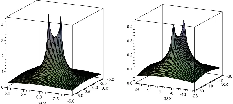
The other interesting example is when the initial and final states are orthogonal to each other (α=π). The smallest timeτp required to evolve from a given initial state|ψiito the orthogonal final state|ψfi is called thepassage time[3,4]. Insertingα=π into equation2.18, we obtain
Let us consider some limiting cases, starting with the saddle point Z = 0 (see Fig. 1). Computation yields τp = π/|Ω|. This can be interpreted as the Hermitian limit of the non-Hermitian system. As can be seen in Fig. 1, the evolution of the non-Hermitian quantum system is faster than that of the corresponding Hermitian system, satisfying the same eigenvalue constraint. Moreover, the passage time τp →0 while|Z| → ∞.
Next, we find thatτp→ ∞ at the pointsZ =±Ω (see Fig.1). To understand this result, we note that Z = Ω implies θ= 0 and thatZ = Ω yieldsθ =π. For both cases, θ= 0 andθ=π, the wave function (2.13) becomes
|ψ(t)i=e−i(λ0±Ω)t/2|ψ ii.
Figure 1. Plot of the passage timeτp versusℜZ andℑZ. Left panel: ℜΩ = 1,ℑΩ = 0.1. Right panel: ℜΩ = 1, ℑΩ = 10. As can be seen from the plots, the singularity occurs at the points Z = ±Ω and
τp=π/|Ω|at the saddle pointZ= 0.
3
Quantum evolution in the vicinity of the exceptional point
In the presence of exceptional points characterized by coalescence of eigenvalues and correspon-ding eigenvectors, non-Hermitian physics differs essentially from Hermitian physics [20,25,26]. Since for the Hermitian operators, the coalescence of eigenvalues results in different eigenvectors, exceptional points do not exist for Hermitian systems. The related degeneracies, referred to as ‘conical intersections’, are known also as ‘diabolic points’. In the context of Berry phase, the diabolic point is associated with the ‘fictitious magnetic monopole’ located at the diabolic point [27, 28]. In turn, the exceptional points are associated with the ‘fictitious complex magnetic monopoles’ [29].
For a two-dimensional system (2.4), the eigenvalues coalesce when Ω = 0. Writing the complex vectorΩasΩ=r−iδ, whererandδare real, one can recast the effective Hamiltonian of equation (2.4) in the form
Hef = λ0
2 11 + 1
2r·σ− i
2δ·σ. (3.1)
As can be seen, the degeneracy points are defined by the following equation:
r2−δ2−2irδcosγ = 0, (3.2)
As follows from equations (2.9)–(2.13), at the exceptional point, the quantum evolution is
Without loss of generality, we further assume δ >0. The computation of the time evolution at the exceptional point then yields
τ = 2
In what follows, imposing the eigenvalue constraint as |Ω| = const, we restrict ourselves by consideration of the orthogonal initial |ψii and final states |ψfi. Substituting α = π into equation (2.13) and taking into account equations (2.15), (2.16), we obtain
|ψ(t)i= exceptional point, there are two different regimes, depending on the relation betweenρ and δ.
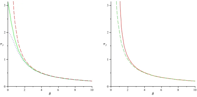
Forρ > δ, we have Ω = pρ2−δ2 >0, and inserting cosθ= (z−iδ)/Ω into equation (3.3), of the non-Hermitian Hamiltonian (3.1) are real, and we obtain the PT-symmetric Hamiltonian widely discussed in the recent literature in connection with the quantum brachistochrone problem [2,5,7,8,9,10,11,12,34,35]. Then, applying (2.18), we get (see Fig. 2)
As can be shown, the passage time τp is bounded above and below as follows: 2/ p
Ω02+δ2 < τp <min{π/Ω0,2/δ}. This improves the estimation of the passage time obtained in [2].
Figure 2. Plot of passage time τp vs. x= δ (Ω0 = 1). Left panel: τp = (2/Ω0) arctan(Ω0/δ) (solid
asymptotically approximated byτ = 2/δ.
Computation of the passage time yields
τp = 2
As seen in Fig. 2, the passage time is bounded below as follows: τp >2/δ, and it follows from equation (3.5) thatτp∼2/δ in the limit Ω0 ≪δ. At the exceptional point, we obtain the same
As an illustrative example, we consider a two-level dissipative system driven by a periodic electromagnetic field E(t) =ℜ(E(t) exp(iνt)). In the rotating wave approximation, after remo-ving the explicit time dependence of the Hamiltonian and the average effect of the decay terms, the Schr¨odinger equation reads [36,37]
i further that V0 >0. The solution of equation (3.6) with this choice ofE can be written as
|u(t)i=C1(t)e−i(ω−iλ)t/2|u↑i+C2(t)ei(ω+iλ)t/2|u↓i,
,denote the up/down states, respectively,
As can be shown, the state|C(t)i satisfies the Schr¨odinger equation
i∂|Ci
∂t =Hr|Ci,
written in a co-rotating reference frame, where the Hamiltonian Hr takes the form
Hr= are two different regimes, depending on the relation between ρ and δ. For ρ > δ, we have a coherent tunneling process
At the exceptional point, Ω0 = 0, and both regimes yield
P↑↑=
This is in accordance with the results obtained by Stafford and Barrett and Dietz et al. [39,
40]. Moreover, the decay behavior predicted by equations (3.7)–(3.8) has been observed in the experiment with a dissipative microwave billiard [40].
We find that forρ > δ, the passage time required to transform the state|u↑iinto the state|u↓i is given by τp = (2/ω0) arctan(ω0/δ). Similarly, forρ < δ, we obtain τp = (2/ω0) tanh−1(ω0/δ). At the exceptional point, for both regimes, the passage time is found to beτp = 2/δ (see Fig.2).
4
Fubini–Study metric on the complex Bloch sphere
and the brachistochrone problem
In this section, we will consider the quantum non-Hermitian brachistochrone problem in the context of the geometric approach developed by Anandan and Aharonov [41]. Let |ψ(t)i and
hψ(t)˜ |satisfy the Schr¨odinger equation and its adjoint equation, respectively:
i∂
∂t|ψ(t)i=H|ψ(t)i, −i ∂
whereHis a non-Hermitian Hamiltonian, and the standard normalization is held,hψ(t)˜ |ψ(t)i=1. We define the complex energy variance as
∆E2=hψ˜|H2|ψi −(hψ˜|H|ψi)2.
Now, applying the Taylor expansion to |ψ(t+ dt)i and using equation (4) and its time derivative, we obtain
hψ(t)˜ |ψ(t+dt)i2= 1−∆E2dt2+O dt3
.
Then, introducing the complex metric as ds2 = 4(1− hψ(t)˜ |ψ(t+dt)i2), we obtain
ds2 = 4∆E2dt2= 4ds2FS, (4.1)
where
ds2FS =hdψ˜|(1−P)|dψi (4.2)
is a natural generalization of the Fubini–Study line element to the non-Hermitian quantum mechanics,P =|ψihψ˜|being the projection operator to the state|ψi. It is easy to show that the complex-valued metric (4.2) is gauge invariant, i.e., it does not depend on the particular choice of the complex phase defined by the map: |ψi →eiα|ψi, hψ˜| →e−iαhψ˜|,α ∈C. We define the
distance between two given states|ψ0iand |ψ1ias
s= 2
Z
C|
∆E(t)|dt, (4.3)
where the integration is performed along a given curveC connecting |ψ0iand |ψ1i.
In the two-dimensional case, the complex-valued Fubini–Study element has a nice geometric interpretation. We define a complex distance between two nearby Bloch vectors n(x) and n(x+dx) by
∆2(x, x+dx) = 1−n(x)·n(x+dx).
Then, applying Taylor expansion,
n(x+dx) =n(x) +∂in(x)dxi+ 1
2∂i∂jn(x)dx
idxj +· · ·,
and using n·n= 1, we obtain, up to second-order terms,
n(x+dx) = 1−dn(x)·dn(x).
This yields
ds2 =dn·dn=gijdxidxj, (4.4)
where gij =∂in·∂jn, and the length of any curveC onSc2 is given by
L(C) =
Z
C|
√
dn·dn|.
Denoting n= (sinζcosν,sinζsinν,cosζ), where ζ, ν∈C, we recast (4.4) as
Finally, using the definition of the complex Bloch vector n=hψ˜|σ|ψi, we find that the metric on the complex Bloch sphereS2
c can be written as
ds2 =dn·dn= 4ds2FS= 4hdψ˜|(1−P)|dψi,
where ds2FS=hdψ˜|(1−P)|dψi is the Fubini–Study line element.
Strictly speaking, gij being a complex-valued tensor does not define a proper metric on the complex Bloch sphere. However, the advantage of this definition is that, contrary to the K¨ahler metric, the complex “metric” (4.4) is invariant under the gauge transformation|ψi → eiα|ψi,
hψ˜| →e−iαhψ˜|, whereα∈C.
For the Hamiltonian (2.20), the straightforward computation yields
2∆E = Ω sinθ, (4.6)
To compare our results with thePT-symmetric model widely discussed in the literature (see, e.g., [6,7,8,9,10,11,12,13,14]), we choose θ=π/2 +iη and assume ℑλ0 =ℑϕ= 0 to write the effective Hamiltonian of equation (2.20) as
Heff = obtain the Hamiltonian of the system in its conventional form (see, e.g., [2,5]):
Heff = becomes the one-sheeted two-dimensional hyperboloidH2with the indefinite metric given by [24]
ds2 = cosh2ρ dν2−dρ2, (4.9)
where −∞< ρ <∞ and 0 ≤ν <2π are the inner parameters onH2. It should be noted that
the interval (4.9) can be obtained from equation (4.5) by the substitutionζ →π/2 +iρ, and we assume ℑν= 0.
The amount of timeτ required to evolve the initial state |ψiiinto the final state|ψfican be found from equation (2.18) by substituting θ=π/2 +iη. The computation yields
τ = 2
and from equation (4.7), we obtain
To study the spin-flip, we choose the initial state as|ψii =|u↑i. Then, substituting α = π into equation (4.10), we find the time interval
τ↓ = 2
Ωarctan 1 sinhη =
2
Ωarctan Ω
δ, τ↑= 2π
Ω −
2
Ωarctan Ω
δ,
necessary for the first spin flip from up to down and back. For all values Ω ∈ [0,∞), we have 2/δ ≤τ↓ ≤π/Ω. Thus, the passage time τp =τ↓ lies below the Anandan–Aharonov lower bound,τ↓ ≤π/Ω for a spin-flip evolution in a Hermitian system [42], andτp reaches its minimum value τmin = 2/δ at the exceptional point. In addition, the total time for a spin-flip evolution,
| ↑i → | ↓i → | ↑i, remains invariant: τ = τ↓ +τ↑ = 2π/Ω. This is in accordance with the results of previous studies [34,10].
Introducing the variable κ = arctan(δ/Ω) = arctan(sinhη), we reproduce our results in the more familiar form, widely known in the literature (see, e.g., [2,3,4,10]):
τ↓ =
π−2κ
Ω , τ↑=
π+ 2κ
Ω .
We see that in the Hermitian limit, η → 0 (δ ≪ Ω) that implies κ → 0, the passage time is given by τp = π/Ω. In the other limiting case η → ∞ (Ω ≪ δ), the angle κ approaches π/2, and τp tends to zero. In terms of variable κ, the relation Ω coshη = ω becomes Ω = ωcosκ. Furthermore, if the energy constraintE+−E−= Ω is held fixed, in order to have the passage to the limitκ→π/2, one must requireω≫Ω. It then follows from the relation Ω2=ω2−δ2 = const that one must require δ ≫Ω.
Similar consideration of the distance between the initial and the final states yields
Lp = 2 coshηarctan
1 sinhη
= π−2κ
cosκ . (4.11)
In the limit κ → π/2, we get Lp →2, and in the Hermitian limit, κ →0, we have Lp → π. It then follows from equation (4.11), that the distance between|u↑i and |u↓i, being measured on the one-sheeted two-dimensional hyperboloid H2 with the indefinite metric of equation (4.9), is
bounded as follows: 2≤Lp ≤π.
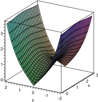
Inserting θ = π/2 +iη into (4.6), we obtain 2∆E = Ω cosη. Then substituting this result into equation (4.1), we find that for the non-Hermitian Hamiltonian (4.8), the evolution speed v = ds/dt is given by v = ω = Ω coshη. Hence, v ≥ vg, where vg = Ω is the speed of the geodesic evolution [24]. Similar consideration of the quantum-mechanical system governed by the Hermitian Hamiltonian yields v = Ω sinθ, and, obviously, v ≤ vg. This proves that non-Hermitian quantum mechanics can be faster than non-Hermitian quantum mechanics. Moreover, since for any complex angle θ, there exists θ0 determined by the equation cosℜθ0 = sinhℑθ0 such that v = |Ω sinθ| ≥ |Ω| = vg if |ℑθ| ≥ |ℑθ0|, this conclusion is applied to an arbitrary non-Hermitian Hamiltonian (see Fig. 3).
Our results are in agreement with those obtained previously by Bender et al. [2]. Howe-ver, interpreting the obtained results for τ requires care. Indeed, as was pointed out by Mostafazadeh [7], to compare the time evolution for the non-Hermitian and Hermitian Hamil-tonians and to conclude in which case the evolution is faster, one should not only impose the same set of constraints for both cases but also fix the geodesic distance between initial and final states.
Figure 3. Plot of the evolution speed|v|/|Ω|versusx=ℜθ andy =ℑθ. As can be observed, for any
θ: 0≤ ℜθ≤π, there exists the angleθ0 such that|v|/|Ω| ≥1, if |ℑθ| ≥ |ℑθ0|.
2∆E =ω and E+−E− = Ω. Then, using the relation coshη =ω/Ω, we find that the passage time can be recast as
τp = 2
Ωarctan Ω
√
ω2−Ω2. (4.12)
As can be observed, under the constraintω= const, the time evolution is bounded by 2/ω ≤ τp ≤ π/ω. Here, the passage time reaches its minimum value τmin = 2/ω at the exceptional point Ω = 0 (η→ ∞). The maximum, τmax=π/ω, is obtained for Ω =ω. Since Ω =ω implies η = 0, this case corresponds to the Hermitian Hamiltonian. Next, we let the energy constraint beE+−E−= Ω = const. Then, as follows from equation (4.12),τp≤π/Ω, and, just as above, the passage time achieves the maximum τmax =π/Ω at the point ω = Ω corresponding to the Hermitian Hamiltonian. For ω≫Ω, we obtain τp ≈2/ω, and τp vanishes in the limitω → ∞.
Similar consideration of the distance between the initial and final states yields
Lp =ωτ = 2ω
Ω arctan Ω
√
ω2−Ω2
and, under the constraint ω = const, we have 2 ≤ L ≤ π. The upper bound Lmax = π, being identical to the geodesic distance between the initial and final states defined either on the Bloch sphere S2 or on the one-sheeted hyperboloid H2 [24], is thus achieved for the Hermitian Hamiltonian (Ω =ω). The lower bound,Lmin = 2, is obtained at the exceptional point (Ω = 0). This agrees with our general conclusions regarding the behavior of the system in the vicinity of the exceptional point (see Section 3). Next, imposing the constraint Ω = const, we obtain the same result 2≤Lp ≤π. The minimum of Lp corresponds to the limit ω≫ Ω, and, just as above, the upper bound is achieved for the Hermitian Hamiltonian (ω = Ω).
This is true in the case of the Hermitian Hamiltonian; however, for a non-Hermitian Hamil-tonian, the situation is quite different [24]. Letni and nf denote antipodal states on the Bloch sphere S2, and mi and mf denote corresponding (antipodal) states on the one-sheeted hyper-boloidH2. Then, the geodesic distanceLgbetweenniandnf calculated over the Bloch sphereS2
is identical to the geodesic distance between mi and mf computed over the one-sheeted hyper-boloid H2 (for detailed calculations, see [24]). Moreover, under the same set of constraints, the
amount of time τg required to evolve ni into nf on the Bloch sphere is equal to that required to evolve mi into mf on H2 by geodesic evolution. This is in accordance with the conclusions made by Mostafazadeh in [7]. However, as we have shown above, in the case of the Hermitian Hamiltonian, τg is the lower bound on the time evolution, and, for the non-Hermitian Hamilto-nian, it yields only the upper bound on the time evolution. Thus, in non-Hermitian quantum mechanics, the evolution of a system is indeed faster than in Hermitian quantum mechanics, subject to the same energy constraint.
5
Conclusion
In this paper, we considered the non-Hermitian quantum brachistochrone problem for the generic non-Hermitian Hamiltonian and focused our attention on the geometric aspects of the problem. We demonstrated that for the generic non-Hermitian Hamiltonian, the quantum brachistochrone problem can be effectively formulated on the complex Bloch sphere Sc2, enabling the latter to be considered as the quantum phase space of the related two-level system. In particular, for the effective non-Hermitian Hamiltonian with a real energy spectrum, the corresponding quantum phase space is represented by the one-sheeted hyperboloidH2.
As noted in [4, 5], in the Hermitian quantum brachistochrone problem, the lower bound on the time evolution interval τ, being proportional to the geodesic distance between the initial and final states on the Bloch sphere, is determined using the Fubini-Studi metric onCP1 ∼=S2.
We have shown that the geodesic distance Lg between antipodal states ni and nf calculated over the Bloch sphere S2 is identical to the geodesic distance between corresponding antipodal states mi and mf calculated over the one-sheeted hyperboloid H2. Moreover, the amount of timeτg required to evolveni intonf on the Bloch sphere is equal to that required to evolvemi intomf onH2 by the geodesic evolution. This is in accordance with the conclusions made in [7]. However, in the case of the Hermitian Hamiltonian,τg is the lower bound on the time evolution, and, for the non-Hermitian Hamiltonian, it yields only the upper bound on the time evolution. Furthermore, while for a quantum-mechanical system governed by the Hermitian Hamiltonian the evolution, speed vis bounded byv≤vg, where vg is the speed of the geodesic evolution, for a non-Hermitian quantum system with the same energy constraint, we havev≥vg. This proves that in non-Hermitian quantum mechanics, evolution can be faster than in Hermitian quantum mechanics [2].
Acknowledgements
References
[1] Carlini A., Hosoya A., Koike T., Okudaira Y., Time-optimal quantum evolution,Phys. Rev. Lett.96(2006),
060503, 4 pages.
[2] Bender C.M., Brody D.C., Jones H.F., Meister B.K., Faster than Hermitian quantum mechanics,Phys. Rev. Lett.98(2007), 040403, 4 pages,quant-ph/0609032.
[3] Brody D.C., Elementary derivation for passage times, J. Phys. A: Math. Gen. 36 (2003), 5587–5593,
quant-ph/0302067.
[4] Brody D.C., Hook D.W., On optimum Hamiltonians for state transformations,J. Phys. A: Math. Gen.39
(2006), L167–L170,quant-ph/0601109.
[5] Bender C.M., Brody D.C., Optimal time evolution for Hermitian and non-Hermitian Hamiltonians, in Time in Quantum Mechanics II, Editor J.G. Muga,Lecture Notes in Phys., Springer, to appear,arXiv:0808.1823.
[6] Assis P.E.G., Fring A., The quantum brachistochrone problem for non-Hermitian Hamiltonians,J. Phys. A: Math. Theor.41(2008), 244002, 12 pages,quant-ph/0703254.
[7] Mostafazadeh A., Quantum brachistochrone problem and the geometry of the state space in pseudo-Hermitian quantum mechanics,Phys. Rev. Lett.99(2007), 130502, 4 pages,arXiv:0706.3844.
[8] Mostafazadeh A., Hamiltonians generating optimal-speed evolutions, Phys. Rev. A 79 (2009), 014101,
4 pages,arXiv:0804.4755.
[9] Bender C.M., Brody D.C., Jones H.F., Meister B.K., Comment on the quantum brachistochrone problem,
arXiv:0804.3487.
[10] G¨unther U., Samsonov B.F., ThePT-symmetric brachistochrone problem, Lorentz boosts and non-unitary operator equivalence classes,Phys. Rev. A 78(2008), 042115, 9 pages,arXiv:0709.0483.
[11] G¨unther U., Samsonov B.F., Naimark-dilatedPT-symmetric brachistochrone,Phys. Rev. Lett.101(2008),
230404, 4 pages,arXiv:0807.3643.
[12] G¨unther U., Rotter I., Samsonov B.F., Projective Hilbert space structures at exceptional points,J. Phys. A: Math. Theor.40(2007), 8815–8833,arXiv:0704.1291.
[13] Martin D., Is PT-symmetric quantum mechanics just quantum mechanics in a non-orthogonal basis?,
quant-ph/0701223.
[14] Rotter I., The brachistochrone problem in open quantum systems, J. Phys. A: Math. Theor. 40(2007),
14515–14526,arXiv:0708.3891.
[15] Weisskopf V.F., Wigner E.P., Berechnung der nat¨urlichen Linienbreite auf Grund der Diracschen Lichttheo-rie,Z. f. Physik63(1930), 54–73.
[16] Weisskopf V.F., Wigner E.P., ¨Uber die nat¨urliche Linienbreite in der Strahlung des harmonischen Oszillators.
Z. f. Physics65(1930), 18–29.
[17] Aharonov Y., Massar S., Popescu S., Tollaksen J., Vaidman L., Adiabatic measurements on metastable systems,Phys. Rev. Lett.77(1996), 983–987,quant-ph/9602011.
[18] Plenio M.B., Knight P.L., The quantum-jump approach to dissipative dynamics in quantum optics, Rev. Modern Phys.70(1998), 101–144,quant-ph/9702007.
[19] Carollo A., Fuentes-Guridi I., Fran¸ca Santos M., Vedral V., Geometric phase in open system, Phys. Rev. Lett.90(2003), 160402, 4 pages,quant-ph/0301037.
[20] Berry M.V., Physics of nonhermitian degeneracies,Czechoslovak J. Phys.54(2004), 1039–1047.
[21] Morse P.M., Feshbach H., Methods of theoretical physics, McGraw-Hill, New York, 1953.
[22] Chu S.-I., Wu Z.-C., Layton E., Density matrix formulation of complex geometric quantum phases in dissipative systems,Chem. Phys. Lett.157(1989), 151–158.
[23] Chu S.-I., Telnov D.A., Beyond the Floquet theorem: generalized Floquet formalisms and quasienergy methods for atomic and molecular multiphoton processes in intense laser fields, Phys. Rep. 390 (2004),
1–131.
[24] Nesterov A.I., An optimum Hamiltonian for non-Hermitian quantum evolution and the complex Bloch sphere,arXiv:0806.4646.
[25] Heiss W.D., Exceptional points of non-Hermitian operators,J. Phys. A: Math. Gen.37(2004), 2455–2464,
[26] Heiss W.D., Exceptional points – their universal occurrence and their physical significance,Czechoslovak J. Phys.54(2004), 1091–1099.
[27] Berry M.V., Quantal phase factor accompanying adiabatic changes, Proc. Roy. Soc. London Ser. A 392
(1984), 45–57.
[28] Berry M.V., Dennis M.R., The optical singularities of birefringent dichroic chiral crystals, Proc. Roy. Soc. London Ser. A459(2003), 1261–1292.
[29] Nesterov A.I., Aceves de la Cruz F., Complex magnetic monopoles, geometric phases and quantum evolution in vicinity of diabolic and exceptional points, J. Phys. A: Math. Theor. 41 (2008), 485304, 25 pages,
arXiv:0806.3720.
[30] Kirillov O.N., Mailybaev A.A., Seyranian A.P., Unfolding of eigenvalue surfaces near a diabolic point due to a complex perturbation,J. Phys. A: Math. Gen.38(2005), 5531–5546,math-ph/0411006.
[31] Mailybaev A.A., Kirillov O.N., Seyranian A.P., Geometric phase around exceptional points,Phys. Rev. A
72(2005), 014104, 4 pages,quant-ph/0501040.
[32] Seyranian A.P., Kirillov O.N., Mailybaev A.A., Coupling of eigenvalues of complex matrices at diabolic and exceptional points,J. Phys. A: Math. Gen.38(2005), 1723–1740,math-ph/0411024.
[33] Mailybaev A.A., Kirillov O.N., Seyranian A.P., The Berry phase in a neighborhood of degenerate states,
Dokl. Akad. Nauk406(2006), 464–468.
[34] Giri P.R., Lower bound of minimal time evolution in quantum mechanics,Internat. J. Theoret. Phys. 47
(2008), 2095–2100,arXiv:0706.3653.
[35] Geyer H.B., Heiss W.D., Scholtz F.G., Non-Hermitian Hamiltonians, metric, other observables and physical implications,arXiv:0710.5593.
[36] Garrison J.C., Wright E.M., Complex geometrical phases for dissipative systems,Phys. Lett. A128(1988),
177–181.
[37] Lamb W.E., Schlicher R.R., Scully M.O., Matter-field interaction in atomic physics and quantum optics,
Phys. Rev. A36(1987), 2763–2772.
[38] Baker H.C., Non-Hermitian quantum theory of multiphoton ionization,Phys. Rev. A30(1984), 773–793.
[39] Stafford C.A., Barrett B.R., Simple model for decay of superdeformed nuclei, Phys. Rev. C 60 (1999),
051305, 4 pages,nucl-th/9906052.
[40] Dietz B., Friedrich T., Metz J., Miski-Oglu M., Richter A., Sch¨afer F., Stafford C.A., Rabi oscillations at exceptional points in microwave billiards,Phys. Rev. E75(2007), 027201, 4 pages,cond-mat/0612547.
[41] Anandan J., Aharonov Y., Geometry of quantum evolution,Phys. Rev. Lett.65(1990), 1697–1700.
[42] Aharonov Y., Anandan J., Phase change during a cyclic quantum evolution, Phys. Rev. Lett. 58(1987),