USING LEAST-SQUARES TO FIND AN APPROXIMATE
EIGENVECTOR∗
DAVID HECKER† AND DEBORAH LURIE†
Abstract. The least-squares method can be used to approximate an eigenvector for a matrix
when only an approximation is known for the corresponding eigenvalue. In this paper, this technique is analyzed and error estimates are established proving that if the error in the eigenvalue is sufficiently small, then the error in the approximate eigenvector produced by the least-squares method is also small. Also reported are some empirical results based on using the algorithm.
Key words. Least squares, Approximate eigenvector.
AMS subject classifications. 65F15.
1. Notation. We use upper case, bold letters to represent complex matrices, and lower case bold letters to represent vectors in Ck. We consider a vector v to be a column, and so its adjointv∗ is a row vector. Hence v∗1v2 yields the complex
dot productv2·v1. The vectorei is the vector having 1 in its ith coordinate and 0 elsewhere, andIn is the n×n identity matrix. We usev to represent the 2-norm on vectors;that is v2 = v∗v. Also, |||F||| represents the spectral matrix norm of a square matrixF, and soFv ≤ |||F||| v for every vector v. Finally, for an n×nHermitian matrixF, we will write each of then(not necessarily distinct) real eigenvalues forFasλi(F), where λ1(F)≤λ2(F)≤ · · · ≤λn(F).
2. The Method and Our Goal. SupposeMis an arbitraryn×nmatrix having λas an eigenvalue, and letA=λIn−M. Generally, one can find an eigenvector for M corresponding to λ by solving the homogeneous system Ax = 0. However, the computation of an eigenvalue does not always result in an exact answer, either because a numerical technique was used for its computation, or due to roundoff error. Suppose λ′ is the approximate, known value for the actual eigenvalueλ. If λ=λ′, then the known matrixK = λ′I
n−M is most likely nonsingular, and so the homogeneous systemKx=0has only the trivial solution. This situation occurs frequently when attempting to solve small eigenvalue problems on calculators.
Let ǫ = λ′−λ. Then K = A+ǫIn. Our goal is to approximate a vector in the kernel ofAwhen only the matrixKis known. We assume thatM has no other eigenvalues within|ǫ|units ofλ, so thatKis nonsingular, and thus has trivial kernel. Letube a unit vector in ker(A). Although we know thatuexists,uis unknown. Let vbe an arbitrarily chosen unit vector inCnsuch thatw=v∗u= 0. In practice, when choosingv, the value ofw is unknown, but ifvis chosen at random, the probability thatw= 0 is zero. LetBbe the (n+ 1)×nmatrix formed by appending the rowv∗
∗Received by the editors 21 March 2005. Accepted for publication 19 March 2007. Handling Editor: Michael Neumann.
†Department of Mathematics and Computer Science, Saint Joseph’s University, 5600 City Avenue, Philadelphia, Pa. 19131 ([email protected], [email protected]).
to K. Written in block form, B=
K v∗
. The system Bx=en+1 is inconsistent,
since any solution must satisfy both Kx = 0 and v∗x = 1, which is impossible since Kx= 0 has only the trivial solution. We apply the least-squares method to Bx=en+1 obtaining a vectorysuch that Byis as close toen+1 as possible. Then,
we normalizey producings=y/y, an approximation for a unit vector in ker(A). This is essentially the technique for approximating an eigenvector described, but not verified, in [1]. Our goal in this paper is to find constantsN1andN2, each independent
ofǫ, and a unit vectoru′∈ker(A), such that
As ≤N1|ǫ|and
(2.1)
u′−s ≤N2|ǫ|.
(2.2)
Note that the unit vectoru′ might depend upon s, which is dependent on ǫ. These inequalities will show that as ǫ→0,As→0 ands gets close to ker(A). Although (2.1) clearly follows from (2.2) by continuity, we need to prove (2.1) first since that inequality is used in the proof of (2.2).
3. Proving Estimate (2.1). The method of least-squares is based upon the following well-known theorem [1]:
Theorem 3.1. Let Fbe anm×nmatrix, letq∈Cm, and letW be the subspace
{Fx|x∈Cn
}. Then the following three conditions on a vector y are equivalent: (i) Fy=projWq
(ii) Fy−q ≤ Fz−q for allz∈Cn (iii) (F∗F)y=F∗q
So, given the inconsistent systemBx=en+1, parts (i) and (iii) of Theorem 3.1
show that the system B∗Bx = B∗e
n+1 is consistent. Let y be a solution to this
system. Withs=y/y, we use the properties ofyfrom part (ii) to prove inequalities (2.1) and (2.2).1
First, using block notation,
B
u
w
−en+1
=
1
wKu
1
wv ∗u−1
=
1
|w|2Ku 2
+ 1 ww−1
2
= 1
|w|Ku=
1
|w|(A+ǫIn)u
= 1
|w|Au+ǫu=
1
|w|ǫu= |ǫ| |w|,
1A quick computation shows thatB∗e
n+1=v, and soyis the solution to a nonhomogeneous
sinceuis a unit vector in ker(A). Hence, by part (ii) of Theorem 3.1 withz= u
w,
|ǫ|
|w| ≥ By−en+1=
Ky v∗y−1
=
Ky2+|v∗y−1|2
≥ Ky=(A+ǫIn)y
≥ Ay − |ǫ| y , by the Reverse Triangle Inequality.
Now, ifAy − |ǫ| y<0, then
As= Ay
y <|ǫ|,
and we have inequality (2.1) withN1= 1.
But, instead, ifAy − |ǫ| y ≥0, then
|ǫ|
|w| ≥ Ay − |ǫ| y, implying
As=Ay
y ≤ |ǫ|
1 + 1
|w| y
.
In this case, we would like to setN1equal to 1 +|w|1y. However,ydepends upon
ǫ. Our next goal is to bound 1 + 1
|w|y independent ofǫ.
Now, sinceKis nonsingular, rank(K) =n. Therefore rank(B) =n. This implies that rank(B∗B) = n, and so B∗B is nonsingular. Since B∗B is Hermitian, there is a unitary matrix P and a diagonal matrix D such that B∗B=P∗DP, where the eigenvalues of B∗B, which must be real and nonnegative, appear on the main diagonal ofDin increasing order. Also, none of these eigenvalues are zero sinceB∗B is nonsingular.
As noted above, B∗e
n+1 = v. The vector y is thus defined by the equation
B∗By=B∗e
n+1=v. Hence,P∗DPy=v, or Py=D−1Pv. Therefore, y=Py=
D−1Pv ≥ min
x=1
D−1Px
= min x=1
D−1x
=
D−1en
=
1 λn(B∗B). And so,
1
y ≤λn(B
∗B), implying
1 + 1
|w| y ≤1 +
λn(B∗B)
|w| .
Our next step is to relateλn(B∗B) toλn(K∗K). Now,
B∗B=
K∗ v
K v∗
Becausev is a unit vector,vv∗ is the matrix for the orthogonal projection onto the subspace spanned byv. Hence, λi(vv∗) = 0 fori < n, andλn(vv∗) = 1. Therefore, by Weyl’s Theorem [2],λn(B∗B)≤λn(K∗K) +λn(vv∗) =λn(K∗K) + 1.
NowK=A+ǫIn, and soK∗K= (A∗+ǫI
n) (A+ǫIn) =A∗A+ (ǫA+ǫA∗) +
|ǫ|2In. ButA∗A, (ǫA+ǫA∗), and|ǫ|2I
n are all Hermitian matrices. Hence, Weyl’s Theorem implies that λn(K∗K) ≤ λn(A∗A) +λ
n(ǫA+ǫA∗) +|ǫ|
2
. Since we are only interested in small values ofǫ, we can assume that there is some boundC such that|ǫ| ≤C. Therefore,λn(K∗K)≤λn(A∗A) +λ
n(ǫA+ǫA∗) +C2.
Next, we need to compute a bound on λn(ǫA+ǫA∗) that is independent of ǫ. Supposepǫ(z) is the characteristic polynomial ofǫA+ǫA∗ andai(ǫ) is the coefficient ofzi inpǫ(z). The coefficients of the characteristic polynomial of a matrix are a sum of products of entries of the matrix, so ai(ǫ) is a polynomial inǫ and ǫ. Therefore,
|ai(ǫ)| attains its maximum on the compact set |ǫ| ≤C. Let mi be this maximum value. Since λn(ǫA+ǫA∗) is a root ofpǫ(z), Cauchy’s bound [2] implies that
|λn(ǫA+ǫA∗)| ≤1 + max{|a0(ǫ)|,|a1(ǫ)|, . . . ,|an−1(ǫ)|} ≤1 + max{m0, m1, . . . mm−1}.
Hence,λn(K∗K)≤λ
n(A∗A) + 1 + max{m0, m1, . . . mm−1}+C2, which is
inde-pendent ofǫ. Finally, we let
N1= 1 +
2 +λn(A∗A) + max{m
0, m1, . . . mm−1}+C2
|w| .
Our argument so far shows thatAs ≤N1|ǫ|, completing the proof of (2.1).2
4. Proving Estimate (2.2). Next, we find u′ and N
2 that satisfy inequality
(2.2). SinceA∗Ais Hermitian, there is a unitary matrixQsuch thatA∗A=Q∗HQ, where H is a diagonal matrix whose main diagonal entries h1, h2, . . . , hn are the real, nonnegative eigenvalues ofA∗A in increasing order. Letl= dim(ker(A∗A)) = dim(ker(A)) >0. Thus,h1 =h2 =· · · =hl = 0, and hl+1 >0. Let t=Qs, with
coordinatest1, . . . tn. Note thatt=Qs=s= 1. Let
tα=
t1
.. . tl
, tβ=
tl+1
.. . tn
, in which caset=
tα tβ
,
where we have writtentin block form. Using this notation, 1 = t2 =tα2+tβ2. Note that
tα 0
is essentially the projection of sonto ker(A∗A) = ker(A), expressed in the coordinates that diagonalizesA∗A.
2Technically, there are two cases in the proof. In the first case, we obtainedN
1= 1. However,
the expression forN1 in Case 2 is always larger than 1, allowing us to use that expression for both
First, we claim that for|ǫ|sufficiently small,tα = 0. We prove this by showing thattβ<1.
Assume that A = O, so that |||A∗||| = 0. (If A = O, the entire problem is trivial.) In addition, suppose that|ǫ|< hl+1
N1|||A∗|||. Then,
|||A∗|||N1|ǫ| ≥ |||A∗||| As ≥ A∗As=Q∗HQs=HQs
=Ht=
n i=1
|hiti|2=
n
i=l+1 |hiti|2
≥hl+1 n
i=l+1
|ti|2=hl+1tβ.
Therefore,
tβ ≤ ||| A∗|||N
1|ǫ|
hl+1
<|||A ∗|||N
1
hl+1
hl+1
N1|||A∗|||
= 1,
completing the proof thattα>0.
Next, we find u′ ∈ ker(A) that is close to s. Since t
α > 0, we can define
z = 1
tα
l
i=1tiei =
1
tαtα
0
, and let u′ = Q∗z. Note that u′ = z = 1. Now,
A∗Au′= (Q∗HQ)(Q∗z) =Q∗Hz=Q∗0=0, and sou′∈ker(A∗A) = ker(A). But
u′−s2=Q(u′−s)2=
Qu′−Qs 2
=QQ∗z−t2=z−t2
= 1
tαtα−tα
−tβ
2 = l i=1 |ti|2
1 tα−
1
2
+ n
i=l+1 |ti|2
= l
i=1 |ti|2
1 tα 2 − 2 tα + 1 − l i=1 |ti|2+
n
i=1 |ti|2
= 1 tα 2 − 2 tα l i=1 |ti|2
+ 1 since n
i=1
|ti|2=t
2 = 1 = 1 tα 2 − 2 tα
tα2+ 1 = 2−2tα
≤2−2tα2= 2(1− tα2) = 2tβ2. Hence,u′−s ≤√2tβ. Next,
Ht=
n i=1
|hiti|2=
n
i=l+1
hi2|ti|2 ≥ hl+1 n
i=l+1
But,
Ht=Q∗Ht=Q∗HQs=A∗As ≤ |||A∗||| As ≤ |||A∗|||N
1|ǫ|.
Putting this all together, we let
N2= √
2|||A∗|||N
1
hl+1
.
Then,
N2|ǫ|= √
2|||A∗|||N
1|ǫ|
hl+1 ≥
√
2 hl+1
Ht ≥ √
2 hl+1
(hl+1tβ) =√2tβ ≥ u′−s,
thus proving inequality (2.2).
5. Further Observations. The formulas we present forN1andN2are derived
from worst-case scenarios, not all of which should be expected to occur simultaneously. Also, the constantsN1andN2depend upon various other fixed, but unknown, values,
such asw=v∗uand |||A∗|||. However, they are still useful, since they demonstrate that, so long asvis chosen such thatv∗u= 0, the least-squares technique works;that is, it will produce a vector close to an actual eigenvector (provided ǫ is sufficiently small). Of course, if one happens to choose v so that v∗u = 0 (which is highly unlikely) and the method fails, one could just try again with a new randomly chosen unit vectorv.
In a particular case, we might want good estimates forAsandu′−s. Using A=K−ǫIn and the triangle inequality produces
As ≤ Ks+|ǫ|.
Hence,Ascan be estimated just by computingKsaftershas been found. (One usually has a good idea of an upper bound on|ǫ|based on the method used to find the approximate eigenvalue.) Similarly, tracing through the proof of estimate (2.2), it can be seen that
u′−s ≤ √
2 (|||K|||+|ǫ|) (Ks+|ǫ|) hl+1
.
Applying Weyl’s Theorem shows that
hl+1≥λl+1(K∗K) +λ1(−ǫK∗−ǫK) +|ǫ|2,
6. Empirical Results. We wrote a set of five computer simulation programs in Pascal to test the algorithm for several hundred thousand matrices. Our goal was to empirically answer several questions:
1. How well does the algorithm work?
2. What effect does the choice of the random vectorv have on the algorithm? 3. What happens as the values ofv∗uapproach zero?
4. In the general case, how often does the value ofv∗uget close to zero? 5. How does the size of the closest eigenvalue toλaffect the error? 6. How does the algorithm behave as the size of the matrixMincreases? 7. Can the algorithm be used to find a second vector for a two-dimensional
eigenspace?
Let us first describe the general method used to generate the matrices to be tested. Since we expect the algorithm to be most useful for small matrices, we restricted ourselves to considering n×n matrices with 3 ≤ n ≤ 9. For simplicity, we used λ = 0. In four of the programs, the dimension of the eigenspace for λ = 0 was 1, in the fifth we specifically made it 2 in order to answer Question #7. In order to get a variety of types of matrices, the programs generated matrices with every possible set of patterns of Jordan block sizes for the Jordan canonical form of the matrix (for example the pattern 1,1,2,2 for a 6×6 matrix represents a 1×1 block for the eigenvalue 0, and then, for other eigenvalues, a 1×1 block, and two 2×2 blocks). The other eigenvalues were chosen using a pseudo-random number generator that created complex numbers whose real and imaginary parts each ranged from−10 to 10. The Jordan matrix was created, and then we conjugated it with a matrix of random complex numbers (generated by the same random number generator). In this way, the program knew all of the actual eigenvalues and corresponding eigenvectors. The number of different matrices generated for each possible block structure ranged from 100 to 5000, depending upon the particular program being run. Our method of generating matrices introduced an eighth question:
8. How does the Jordan block pattern of the matrix effect the error?
Next, in all cases, we used λ′ = 0.001 as the estimate for the actual eigenvalue 0. Although in practice, the error in λ′ will be much smaller since it is typically caused by round-off error in some other computation, we used this larger value for two reasons. First, we wanted to be sure that error caused by the error in λ′ would dominate natural round-off error in our computer programs, and second, we wanted to allow forv∗uto be significantly smaller than the error inλ′.3
The random vectorvused in the algorithm was created by merely generating n random complex numbers for its entries, and then normalizing the result to obtain a unit vector.
We measured the error in the approximate unit eigenvectorsby first projectings onto the actual eigenspace forλ= 0, normalizing this result to get a unit eigenvector u′, and then computingu′−s. If the magnitude of the error in each coordinate of
sis about 0.001 (the error inλ), then the value ofu′−s would be about 0.001√n. Thus, we used this level of error as our standard for considering the algorithm to have successfully found an approximate eigenvector. We deemed the error to be large if it exceeded 0.001√n. We also recorded the absolute value of the eigenvalue closest to zero, in order to answer Question #5.
Let us consider the results of our simulations:
1. How well does the algorithm work? (Simulation 1)
When the algorithm was used on 325,000 matrices of varying sizes and Jordan block patterns with a randomly generated vectorv, the error exceeded 0.001√n in only 0.86% (2809/325000) of the matrices. The error had a strong negative correla-tion (−0.7) with the size of the next smallest eigenvalue, indicating a strong inverse relationship between the size of this eigenvalue and error in the algorithm. This is exactly what we should expect, considering thathl+1 appears in the denominator of
N2 in theoretical error estimate (2.2). The mean value of the size of the smallest
eigenvalue when the error exceeded 0.001√n was less than 0.7, as compared to a mean of over 4 for the other trials. (This answers Question #5.) No correlation was found between the error and the absolute value ofv∗ufor this general case. In this simulation, the smallest value|v∗u|observed was 0.0133.
2. What effect does the choice of the random vector vhave on the algorithm? (Simulation 2)
The goal of this simulation was to evaluate the variability in the error insif the initial random vectorv is varied. For each of 13,000 matrices, 200 different random vectorsvwere selected and the algorithm was executed, for a total of 2,600,000 trials. In general, for each of the 13,000 matrices, there was very little variation in the error insover the 200 vectors forv. The range of errors in a given matrix was as small as 9.0×10⁻¹²and as large as 0.0225. The average standard deviation of error per matrix
was at most 1.45×10⁻⁵. Since simulation 2 had more trials than simulation 1, the
minimum value of |v∗u| in simulation 2 (0.00001) was smaller than in simulation 1 (reported above). However, the percent of trials in which the error exceeded 0.001√n was still only 0.90%. Again, the large errors were associated with low values for the size of the smallest eigenvalue.
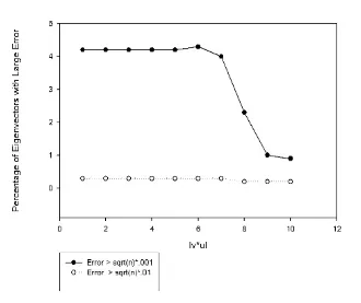
3. What happens as the values ofv∗uapproach zero? (Simulation 3)
In this simulation, for each of 6,500 matrices, 200 vectors v were specifically selected so that|v∗u|approached zero. Hence,vwas not truly random. (This yields a total of 1,300,000 trials.) The value of|v∗u| ranged from 1.39×10⁻¹⁷ to 0.0969.
Errors insthat exceeded 0.001√nwere observed in 3.48% of the trials (as compared to 0.86% and 0.90% in simulations 1 and 2). The trials were grouped by value of
|v∗u|into 10 intervals, labeled 1 through 10 in Figure 6.1: (0, 10−14), (10−14, 10−12),
(10−12, 10−10), (10−10, 10−8), (10−8, 10−6), (10−6, 10−5), (10−5, 10−4), (10−4, 10−3),
(10−3, 10−2), (10−2, 1.0). The percent of large errors is approximately 1% for |v∗u| between 0.001 and 1. The rate increases to 2.3% for values between .0001 and.001 and then to 4% for values between.0001 and.00001. The rate ranges between 4.18% and 4.25% as|v∗u| decreases toward 0.
per interval of values for|v∗u|are graphed in Figure 6.1.
Fig. 6.1.A comparison of the error rates by|v∗u|
4. In the general case, how often does the value ofv∗uget close to zero? A value for|v∗u|less than 0.001 (Categories 9 and 10, above) never occurred in simulation 1 and was observed in only 20 cases (out of 2,600,000) in simulation 2. Thus, we conclude that if the vector v is truly chosen at random, as in simulations 1 and 2, the value of |v∗u| is rarely an issue. The effect of a small value of |v∗u| causing large error was really only seen in simulation 3, in which v was not chosen randomly, but rather|v∗u|was forced to approach zero.
5. How does the size of the closest eigenvalue toλeffect the error?
This question was answered by simulation 1, in which we found a strong inverse relationship between the size of this eigenvalue and error in the algorithm, as was expected.
slight increase in the percentage of cases with large error asn increases. Because of the strong inverse relationship between error and the size of the closest eigenvalue, we suspect that this small increase in error is mostly an effect of the random generation method used for choosing the matrices.
7. Can the algorithm be used to find a second vector for a two-dimensional eigenspace? (Simulation 4)
In this simulation, the matrices ranged from 4×4 to 9×9 in size, and we generated 5000 matrices for each possible Jordan block pattern having at least two Jordan blocks, for a total of 895,000 matrices. Two of the blocks in each matrix were assigned to the eigenvalue λ = 0. Thus, in some cases, zero was the only actual eigenvalue. Eigenvalues corresponding to the other blocks were assigned at random. For each matrix we computed the following:
• The size of the smallest (nonzero) eigenvalue, if it existed.
• An approximate unit eigenvector u1 and the error from its projection onto
the actual eigenspace forλ= 0.
• The norm ofAu1, to help test theoretical Estimate (2.1).
• A second approximate unit eigenvector,u2, found by choosing a second
ran-dom vectorvin the algorithm.
• The error foru2and the value ofAu2.
• The length of the projection of u2 onto u1, to measure how different the
two approximate eigenvectors were;that is, how close isu2 to being a scalar
multiple ofu1? We considered a value>0.9 to be unacceptable, and between
0.8 and 0.9 to be moderately acceptable, but not desirable.
• A unit vector u3 found by normalizing the component ofu2 orthogonal to
u1. (Sou1andu3would form an orthonormal basis (approximately) for the
two-dimensional eigenspace.)
• The error foru3and the value ofAu3.
• Another approximate unit eigenvector, u4, found by choosing the random
vectorv in the algorithm to be orthogonal to the vectoru1, thus making it
less likely foru4 to be a scalar multiple ofu1. • The error foru4and the value ofAu4. • The length of the projection ofu4ontou1.
• A unit vector u5 found by normalizing the component ofu4 orthogonal to
u1.
• The error foru5and the value ofAu5.
These were our results:
• In assessingu1, the error exceeded 0.001√nin only 0.2% (1800) of the 895,000
matrices. The value ofAu1 was always within the acceptable range.
Sim-ilarly, for u2, the error exceeded 0.001√nin 0.104% (933) of the matrices.
The value ofAu2was also always within the acceptable range. Since there
is no real difference in the methods used to generateu1andu2, this amounts
to 1,790,000 trials of the algorithm with only 2733 cases of large error. This is comparable to the general results for the algorithm found in simulation 1, in which the eigenspace was one-dimensional.
87.6% of the cases, and greater than 0.9 in 81.0% of the cases. Hence,u2was
frequently close to being a scalar multiple ofu1.
• The error inu3exceeded 0.001√nin only 0.4% of the matrices (3597/895000).
The value ofAu3was always within the acceptable range. Thus, while this
is still a relatively small percentage of cases, the percentage of large errors almost quadrupled fromu2 tou3.
• The error in u4 exceeded 0.001√nin 0.24% of the matrices (2111/895000),
with Au4 always being within the acceptable range. The length of the
projection ofu4ontou1exceeded 0.8 in 39.0% of the cases, and exceeded 0.9
in 24.5% of the cases, a large improvement overu2.
• The vector u5, orthogonal to u1, had large error in 0.47% of the cases
(4203/895000), and had small error inAu5in all cases.
• We computed the Spearman rank-order correlation between the size of the smallest eigenvalue and the error of each vector. Surprisingly, for matrices 5×5 and larger, there was no correlation found – the correlation coefficients ranged from−0.052 to 0.052. For the 4×4 matrices, there was a low negative relationship. Correlation coefficients with each of the five error terms ranged from −0.314 to −0.231. However, further analysis of the error in u4 found
that for those matrices in which the error in the estimated eigenvector was greater than 0.001√n, the size of the smallest eigenvalue was less than 1 in 74.5% of the matrices, greater than 1 in 14.7% of the matrices, while 10.8% of these large errors were from matrices in which 0 was the only eigenvalue. In running this simulation there were 13 cases in which, while computing either u1, u2, oru4, the program reported that the matrixB∗B was singular, and so the
desired vector could not be computed. (The program actually arbitrarily changed a 0 in a pivot position to a 1 and continued on anyway, with remarkably good results.) Twelve of these 13 cases occurred with matrices in which there were only two Jordan blocks, and soλ= 0 was the only eigenvalue. The remaining case was a 5×5 matrix with a 1×1 and a 3×3 Jordan block for λ= 0, and a single 1×1 block for some other eigenvalue (having absolute value about 4.96).
From simulation 4, we came to the conclusion that the algorithm works equally well for cases in which the eigenspace is two-dimensional, and that the preferred method for finding a second eigenvector not parallel to the first is to choose a random vector v for the algorithm that is orthogonal to the first approximate eigenvector found, as done in the computation ofu4.
8. How does the Jordan block pattern of the matrix effect the error? (Simulation 5)
In this simulation, we allowed the size of the single Jordan block for the eigenvalue λ= 0 to range from 1 to (n−1). Now, a generic matrix should be diagonalizable, and so the Jordan block pattern will have all 1×1 blocks. We compared the typical error in this generic block pattern with the error observed in other non-generic block patterns. Our results indicated that there was no change in error if non-generic block patterns are used rather than the generic block pattern.
corresponding eigenvalue is known.
Acknowledgments. We would like to thank William Semus for his helpful work at the beginning of this project computing many examples by hand.
REFERENCES
[1] S. Andrilli and D. Hecker.Elementary Linear Algebra, third edition. Elsevier Academic Press, Burlington, 2003.