T H E J O U R N A L O F H U M A N R E S O U R C E S • 45 • 1
Workers
Alexander Hijzen
Richard Upward
Peter W. Wright
A B S T R A C T
We use a new, matched worker-firm dataset for the United Kingdom to es-timate the income loss resulting from firm closure and mass layoffs. We track workers for up to nine years after the displacement event, and the availability of predisplacement characteristics allows us to implement dif-ference-in-differences estimators using propensity score matching methods. Income losses during the first five years after the displacement event are in the range 18–35 percent per year for workers whose firm closes down, and 14–25 percent for workers who exit a firm which suffers a mass lay-off. These losses are largely due to periods of nonemployment, which is consistent with previous work from Europe, but contrasts with that from the United States.
I. Introduction
Modern labour markets are continuously in motion. The burgeoning literature on job creation and destruction has documented high levels of job turnover
Alexander Hijzen is an economist at the OECD. Richard Upward is an associate professor and Peter W. Wright is a reader in labour economics at the School of Economics, University of Nottingham, NG7 2RD, UK. All are research fellows of the Leverhulme Centre for Research on Globalisation and Eco-nomic Policy, University of Nottingham and acknowledge financial support through the Leverhulme Trust (Grant No. F/00 114/AM). This work contains statistical data from ONS, which are Crown copy-right and reproduced with the permission of the controller of HMSO and Queen’s Printer for Scotland. The use of the ONS statistical data in this work does not imply the endorsement of the ONS in relation to the interpretation or analysis of the statistical data. The authors thank the staff of the Virtual Micro-data Laboratory (VML) at the Office for National Statistics for their help in accessing the Micro-data. The data used in the paper is held at the VML of the Office of National Statistics. Researchers may apply to use the data, but must access it from one of the VML sites (currently London, Belfast, Glasgow, New-port, and Titchfield). All of the command files needed to replicate the results here are in a publicly accessible folder within the VML lab should other researchers require them. Details regarding access and the command files used in the analysis can be obtained beginning August 2010 through July 2013 from Peter Wright, School of Economics, University of Nottingham, NG7 2RD, UK
Peter.Wright@nottingham.ac.uk.
[Submitted July 2007; accepted October 2008]
in developed economies, due to firm entry, growth, exit and decline. While this process is a key source of productivity growth, there are likely to be significant adjustment costs. In particular, workers must move from those jobs which are de-stroyed to those which are created. Many academic studies, especially in the United States, have attempted to quantify the costs of worker displacement in terms of wage loss and unemployment. Most of these studies have suggested that the costs of displacement are large and long-lasting. More recently, efforts have been made to provide estimates for workers in other parts of the world, several of which have appeared in Kuhn (2002). But surprisingly, very little is known about these costs for workers in the United Kingdom.
In this paper we provide estimates of the income loss resulting from firm closure and mass-layoffs using a newly available matched worker-firm dataset. Our data come from linking a 1 percent sample of U.K. workers to a large panel (effectively a census from 1997 onwards) of firms in the United Kingdom from 1994–2003. We are able to track workers for up to nine years after the displacement event. The availability of predisplacement characteristics allows us to implement difference-in-differences estimators which use both regression and matching methods.
This paper makes the following contributions. First, we provide the first estimates from a large random sample of workers of the income costs of displacement in the United Kingdom. Second, we focus on the relative contributions of periods of un-employment and wage changes to the total costs of displacement. The U.S. literature has found that losses are primarily caused by lower wages in postdisplacement jobs, whereas evidence from France and Germany finds almost no wage losses for those who reenter employment. Third, the paper analyzes the role of four modelling de-cisions for the measurement of displacement costs: the choice of the relevant treat-ment and comparison groups; the choice of the definition of displacetreat-ment; the choice of estimation method; and the measure used for out of work income. Not only does this help us to establish the robustness of our results, but it also allows us to better identify the nature of displacement costs.
Our estimates suggest that the income costs of displacement in the United King-dom over the five years after the event are in the range 18–35 percent per year for workers whose firm closes down, and 14–25 percent for workers who exit a firm which suffers a mass layoff. We find that the choice of comparison group can have a large effect on the estimated cost, but that the choice of estimation method is less important. Conclusions about the longevity of income losses also depend on the choice of comparison group. In line with estimates for other European countries,1 we find that actual wage losses are relatively small, although the extent of wage losses depends on how long it takes displaced workers to reenter employment. Most income losses come from periods of nonemployment.
In Section II we briefly review recent estimates of the income losses of displaced workers. The data construction process is described in Section III. The methodolog-ical issues are explained in Section IV and results are presented in Section V. Section VI concludes.
II. Previous estimates
There is a large literature which estimates the effects of displacement on workers’ incomes, mostly from the United States. A number of these studies use the Displaced Workers Supplement (DWS).2These studies compare in-work income before and after a group of workers experience displacement. They are limited to a before and after comparison because the DWS only contains data on displaced work-ers, so an explicit control group is not available.
Following Ruhm (1991) and Jacobson, LaLonde and Sullivan (1993), an alter-native strategy is to combine the before and after comparison with a similar com-parison for a control group of workers who have not experienced displacement. This is a form of the difference-in-differences estimation method, which in this case is implemented by using a fixed-effects estimator. These studies use data either from representative household surveys such as the PSID3or administrative data.4
The influential paper of Jacobson, LaLonde, and Sullivan (1993) (henceforth JLS) suggests that there are large and long-lasting effects of displacement on workers’ incomes. Even six years after separation, JLS estimate that the incomes of high-tenure workers are some 25 percent lower than a control group. JLS do not attribute this loss in income to higher rates of nonemployment.5There are three points to note with regard to this result. First, the sample JLS use includes only workers who have positive in-work incomes in each calendar year, and so excludes individuals with long spells of unemployment. Second, “nonemployment” is defined as an entire quarter with zero in-work income, and so apparent wage losses might in fact be quarters during which an unemployment spell ended, started or both.6 Third, one should also note that JLS restrict their sample to those workers who have had at least six or more years of tenure by the beginning of 1980. Their sample of displaced workers from 1980–86 therefore consists of high tenure workers who might be expected to have higher income losses than a random sample of all workers. We investigate this issue in our data.
Schoeni and Dardia (1997) use a similar methodology to examine California in the 1990s. Although they show that most of the large initial drop in income is due to a drop in employment (only 70 percent of those displaced have nonzero in-work income in the quarter following displacement), three years after displacement em-ployment rates are about 90 percent, confirming JLS’s finding that most of the long-run income loss is a genuine wage loss for those in employment.
Hildreth, von Wachter, and Handwerker (2005) are able to link State administra-tive data (such as that used by JLS) with the Displaced Workers Supplement.
Cor-2. See, inter alia, Podgursky and Swaim (1987), Kruse (1988), Kletzer (1989), Addison and Portugal (1989), Topel (1990), Gibbons and Katz (1991), Carrington (1993), Neal (1995), Kletzer (1996), and Farber (2003).
3. Examples include Ruhm (1991) and Stevens (1997).
4. Examples include Jacobson, LaLonde, and Sullivan (henceforth JLS); Stevens, Crosslin, and Lane (1994); Schoeni and Dardia (1997).
5. “Thus, the substantial earnings losses observed . . . are largely due to lower earnings for those who work, rather than an increase in the number of workers without . . . earnings” (p.697).
recting for measurement error, they estimate a significantly smaller cost of job loss (12–16 percent of the predisplacement wage).
More recently, efforts have been made to provide estimates for workers in other parts of the world, several of which have appeared in Kuhn (2002).7These studies find much smaller wage losses than those estimated by JLS and other earlier U.S. studies. Borland et al. (2002) is the United Kingdom contribution to this volume, and is the only other U.K. study which looks at the effects of displacement directly.8 Borland et al. (2002) use a sample of workers from the British Household Panel Survey (BHPS) over the period 1991–96. Displacement is self-reported: individuals are asked the reason why they left their last job. It is difficult to compare Borland et al.’s results with those from the U.S. literature because they focus only on indi-viduals who return to employment before the end of the sample period, and also they use a before-and-after methodology rather than difference-in-differences. Nev-ertheless, it is noticeable that wage losses are much smaller than those estimated by JLS. The raw wage penalty is estimated to be between 2 and 14 percent, and wage falls are limited to those who experience some time out of employment after the displacement event. It is not possible to calculate longer-run losses with these data, partly due to the small sample size.9
Recently, studies of worker displacement have begun to use the “potential out-comes” approach associated with Rubin. Here, displaced workers are explicitly matched to observably equivalent nondisplaced workers. For example, Huttunen, Møen, and Salvanes (2006), Eliason and Storrie (2006) and Ichino et al. (2006) use large administrative datasets for Finland, Sweden, and Austria respectively. Huttu-nen, Møen and Salvanes (2006) find that displacement effects on income for those who do not leave the labour force are quite small, around 5 percent, which is con-sistent with other results for European countries reported above. The employment effects of displacement appear to be larger, with a significant impact on the proba-bility of leaving the labour force permanently. However, Eliason and Storrie (2006) find that the size of any income loss is crucially related to the state of the macro-economy, because recently displaced workers are more at risk from subsequent shocks.
Thus, the little evidence we have suggests that wage losses are much smaller in Europe than in the United States, although, even in the United States, estimates vary widely. This might be due to differences in methods and samples, but it is also possible that it reflects genuine differences in labour markets between the United States and Europe. For example, longer duration unemployment benefits might be associated with smaller wage losses but longer spells of job search following
dis-7. Bender et al. (2002) and Burda and Mertens (2001) provide estimates for France and Germany; Abbring et al. (2002) compare estimates for the United States and the Netherlands, for example.
8. Borland et al. (2002) analyse a small sample of self-reported displaced workers. A number of recent U.K. studies have provided estimates of the effect of spells of unemployment on subsequent in-work income. See, for example, Arulampalam (2001), Gregory and Jukes (2001) and Nickell, Jones and Quintini (2002). Of course, these papers do not provide a comparable estimate of the effect of displacement because being unemployed is not the same as being displaced.
placement. However, existing estimates for the United Kingdom are based on much smaller samples and use a different methodology.
III. Data
In order to evaluate the impact of firm closure or mass-layoff we need longitudinal information on workers linked to the firms for which they work. For each firm we require a measure of employment and an indicator of firm closure. Survey data on individuals or households (such as the BHPS in the United Kingdom or the PSID in the United States) typically do not record the identity of workers’ employers, nor are they able to identify firm closure. We therefore use various datasets made available at the Virtual Microdata Laboratory of the Office for Na-tional Statistics to construct a new matched worker-firm dataset for the United King-dom.
TheNew Earnings Survey(NES) is a random sample of 1 percent of employees whose pay has ever been above the level at which National Insurance becomes payable. The last two digits of an individual’s National Insurance number are used to select the sample, and so it can be linked across time to form a panel. Information is collected from employers for a reference week in the April of each year. Firms can be identified by a reference number, although in some years this information is not available for all workers. Individuals in the NES may hold more than one job, and to simplify the subsequent analysis we keep only the highest-paid job for each individual in each year. We also remove the (very small) number of individuals with inconsistent measures of age and sex. We remove individuals who are aged over 60 in 2003 or less than 20 in 1993. The resulting sample has slightly over 150,000 observations (workers) per year.
The Inter-Departmental Business Register (IDBR) is a list of U.K. firms main-tained by the ONS. A comprehensive description can be found in Office for National Statistics (2001). The IDBR linking fileis a subset of the IDBR which contains the link between firm reference numbers and the firm identifier in the NES.
The Annual Business Inquiry (ABI) is an annual survey of firms which, since 1994, has been sampled from the IDBR. The “selected sample” of the ABI is a census of all large firms with 250 or more employees, and a sample of smaller firms. The “nonselected sample” are those firms in the sampling frame which were not selected for the survey (see Jones (2000) for a more detailed description). The An-nual Respondents’ Database(ARD) contains the information from the ABI for each year.
The ARD can be analysed at various levels of aggregation, but it is most straight-forward to link the data at the level of the firm.10The resulting linked dataset is an unbalanced annual panel of employees. For each employee we observe their gross weekly pay including overtime payments yit and a set of characteristicsxit which
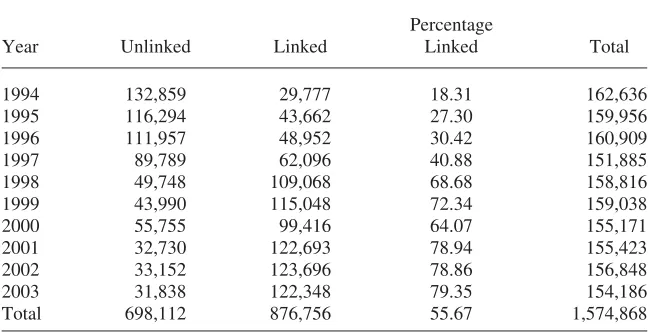
includes age, sex, industry and occupation. If an individual is successfully linked we observe their employer’s identification number, employment and whether their employer existed at tⳭ1. Basic sample sizes of the linked dataset are shown in
Table 1. Note that up to 1997 only a minority of individuals in the NES can be linked. For 1994–96 this is because the firm data only covered the manufacturing sector. For 1997 the low linking rate is because firm reference numbers are missing in the NES.
In common with most administrative datasets, the NES does not record whether a change of employer or a movement from employment to nonemployment is the result of an employer-initiated separation (for example a displacement) or a volun-tary movement by the employee (for example a quit). We therefore use information from the firm-level data to define displacement. Our first indicator is based on firm closure: an individual is displaced betweentandtⳭ1 if their employer attno longer
exists attⳭ1.11Our second indicator is based on changes in employment: an indi-vidual is displaced between t and tⳭ1 if they leave their current employer and employment falls by more than 30 percent between tandtⳭ1.12The mass-layoff sample includes the firm closure sample by definition.
To construct the estimation sample, we proceed as follows. We separate the sam-ple into a control group and a treatment group for each possible year of displacement. For example, the “1998 treatment group” comprises individuals who experienced displacement between the reference weeks in 1998 and 1999, while the “1998 control group” are those who did not experience displacement between 1998 and 1999. Each control and treatment group is a balanced panel from 1994–2003. For estimation purposes it is useful to define a measure of time relative to the displacement event, t*. For example, we definet*⳱0 in 1998 for the 1998 treatment and control groups.
All cohorts are then stacked to create a data set which follows nine cohorts (1994– 2002) of control and treatment groups from t*⳱ⳮ8 to t*⳱9. This allows us to
estimate the pooled effect of displacement at each value of t* across all years of displacement.13
As noted in Section II, comparisons of estimated displacement costs from the extant literature are cumbersome because of numerous methodological differences. For example, some authors exclude periods of nonemployment and focus only on observed wage losses (Borland et al. 2002, Bender et al. 2002). This implies a nonrandom and almost certainly nonrepresentative sample. Furthermore, many pre-vious studies have concentrated on the income losses of specific groups of workers. JLS, for example, consider only workers with six or more years of tenure. The estimated income losses for high tenure workers may be substantially higher than
11. We perform checks to verify that the disappearance of a firm reference number in the ARD is actually a firm exit, rather than simply a recoding of the reference number. We compare the disappearance of the firm identifier in the ARD and the NES. In about 20 percent of cases a firm identifier which disappears from the ARD is not associated with a change in the NES firm identifier, which suggests that these firms did not in fact exit. We therefore code these as nonexits.
Table 1
Number of workers with linked firm reference numbers
Year Unlinked Linked
Percentage
Linked Total
1994 132,859 29,777 18.31 162,636
1995 116,294 43,662 27.30 159,956
1996 111,957 48,952 30.42 160,909
1997 89,789 62,096 40.88 151,885
1998 49,748 109,068 68.68 158,816
1999 43,990 115,048 72.34 159,038
2000 55,755 99,416 64.07 155,171
2001 32,730 122,693 78.94 155,423
2002 33,152 123,696 78.86 156,848
2003 31,838 122,348 79.35 154,186
Total 698,112 876,756 55.67 1,574,868
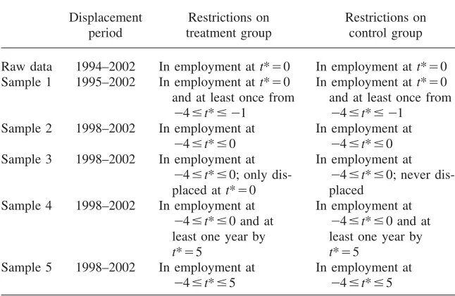
for a randomly selected worker due to the accumulation of firm-specific skills or because of higher match quality. Some studies have also imposed various restrictions on the control groupafterdisplacement. JLS, for example, consider a control group who remain in employment in the same firm throughout the sample period. In order to enhance the comparability and robustness of our results we construct five different samples which vary in their treatment of spells of nonemployment and the appro-priate comparison groups. The definition of each of these samples is given in Table 2.
Sample 1uses information on all displaced and nondisplaced individuals who are observed in employment at t*⳱0, and in employment in at least one year in the
preceding four years. We make this restriction to remove individuals who may ap-pear only once in the data, possibly because they received a temporary national insurance number att*⳱0.
Sample 2only includes individuals who are employed in all five years leading up to displacement. This sample will exclude workers who only recently began a spell of employment and will therefore include a higher proportion of longer-tenure work-ers.
Sample 3 modifies Sample 2 slightly by excluding individuals who experience multiple displacements, and by restricting the control group to comprise those who never experience displacement. This sample enables us to see whether repeated dis-placements add to the total effect of an initial displacement (Stevens 1997).
Table 2
Samples used in the analysis
Displacement period
Restrictions on treatment group
Restrictions on control group
Raw data 1994–2002 In employment att*⳱0 In employment att*⳱0
Sample 1 1995–2002 In employment att*⳱0 and at least once from
ⳮ4ⱕt*ⱕⳮ1
In employment att*⳱0 and at least once from
ⳮ4ⱕt*ⱕⳮ1
Sample 2 1998–2002 In employment at
ⳮ4ⱕt*ⱕ0
In employment at
ⳮ4ⱕt*ⱕ0
Sample 3 1998–2002 In employment at
ⳮ4ⱕt*ⱕ0; only
dis-placed att*⳱0
In employment at
ⳮ4ⱕt*ⱕ0; never
dis-placed
Sample 4 1998–2002 In employment at
ⳮ4ⱕt*ⱕ0 and at least one year by t*⳱5
In employment at
ⳮ4ⱕt*ⱕ0 and at least one year by t*⳱5
Sample 5 1998–2002 In employment at
ⳮ4ⱕt*ⱕ5
In employment at
ⳮ4ⱕt*ⱕ5
Finally,Sample 5includes only periods of employment. This sample can be used to make pure wage comparisons between the treatment and control groups, rather than income comparisons.
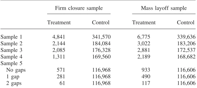
Table 3 summarizes the size of the treatment and control groups for each of the samples used in the paper. Sample sizes vary substantially, mainly because imposing restrictions on predisplacement events removes earlier cohorts from the data.14 Sam-ple 5 is split according to the length of the ‘gap’ until reemployment. Of the 2,144 displaced workers in Sample 2, only 571 are observed in every yeart*0; 281 are observed in every yeart*1 and so on.
Samples 1–4 all rely on the assumption that nonappearance in the NES reflects a spell of nonemployment, rather than a spell of employment which is not picked up in the data. The NES is a statutory survey with high response rates, so this assump-tion will be accurate in most cases. This is also the same assumpassump-tion made by JLS in their administrative data. However, nonappearance of an individual in the NES might also be caused by spells of self-employment or employment which falls below the income tax threshold.15 Temporary nonappearance can also be caused by the failure to locate an individual’s employer, although this will manifest itself as a
14. For example, Samples 2–5 exclude the 1994–97 cohorts because these workers are not observed for four years before the displacement event.
Table 3
Number of displacements in the linked data
Firm closure sample Mass layoff sample
Treatment Control Treatment Control
Sample 1 4,841 341,570 6,775 339,636
Sample 2 2,144 184,084 3,022 183,206
Sample 3 2,085 176,328 2,881 172,537
Sample 4 1,311 169,560 2,189 168,682
Sample 5
No gaps 571 116,968 933 116,606
1 gap 281 116,968 490 116,606
2 gaps 61 116,968 117 116,606
short-lived disappearance from the data, and will not affect long-run estimates of income losses.16
For periods of nonemployment we follow two approaches to the specification of out of work income. Firstly, we allocate these individuals standard rates of the Jobseekers’ Allowance, the benefit payable to those actively seeking work.17The value of Jobseekers’ Allowance is similar to other benefits paid to individuals with-out work, such as Income Support and Incapacity Benefit. This allows us to assess the effect of displacement on workers’ well-being. Secondly, in common with JLS, we assume an income of zero for periods of nonemployment. This allows a better comparison with the existing literature.
IV. Methods
In common with the literature on policy evaluation,18 we treat a worker displacement as a “treatment” which may have some impact on workers’ future labour market outcomes. The most important issue is how to construct the counterfactual: what would have happened, on average, to a displaced worker had they not been displaced.19
In the absence of a genuine experiment which randomly assigns individuals into the treatment and control groups, there are essentially two methods for constructing counterfactual income. The first is to use income of the treatment group fort*ⱕ0, and then to compare income before and after displacement. As noted by JLS, this
16. Temporary nonappearance may occur if an individual starts a job in the period between the sampling of the firms in February and the survey in April.
17. Rates are taken from www.statistics.gov.uk/STATBASE/Expodata/Spreadsheets/D3989.xls. 18. See Blundell and Costa Dias (2002) for a recent summary.
comparison may be misleading. First, it ignores factors (such as macroeconomic shocks) which cause changes to income regardless of displacement. Second, it ig-nores income growth which would have occurred anyway. Finally, if income de-clines before displacement,20before and after estimates can be sensitive to the choice of time period.
The second method is to use the income of a control group to construct counter-factual income. Much of the literature on displacement recognises that the event is likely to be nonrandom, and so some care must be taken in defining the control group.21Nonrandom assignment is likely to be a particular problem for our mass-layoff sample, since not all workers in a firm lose their job. Employer selection suggests that those workers with lower productivity will be displaced, while em-ployee selection suggests that those workers whose outside job prospects are better will choose to leave. Even in the case of firm closure, it may be that those workers who remain in the firm untilt*⳱0 are a nonrandom sample of all those in the firm
at the point where closure became public knowledge.22
If assignment is nonrandom with respect to a permanent unobserved component of income one can measure the difference between the control and treatment groups in their before—after difference in income, using a difference-in-differences (DiD) estimate.
A generalisation of DiD allows for an individual unobserved permanent income component (or fixed effect) rather than a group fixed effect. The choice of predis-placement time period is important: if one chooses, for example,t*⳱ⳮ1 then it is
possible that this does not reflect permanent income differences between the groups, but rather some genuine predisplacement dip in income. We therefore choose as a “base period” the average difference in income between the two groups for
ⳮ8ⱕt*ⱕⳮ4. This gives us our basic estimating equation:
9 9
k k k k
y ⳱aⳭ ␥ T Ⳮ ␦ D•T Ⳮε
(1) it i
兺
it兺
i it itk⳱ⳮ8 k⳱ⳮ3
whereyitis the log of income for individualiat timet. EachTkit is a dummy equal
to one ift*⳱k and zero otherwise.Diis a dummy equal to one if the individual is
displaced, and zero otherwise. Equation 1 can be estimated by taking within-i de-viations from means, or differencing, and is essentially that estimated by JLS.23
If selection into the treatment and control groups is on the basis of the unobserved permanent income component, then Equation 1 will yield consistent estimates of the expected income loss. However, it is likely that there are also time-varying
char-20. The so-called “Ashenfelter dip,” from Ashenfelter (1978).
21. For example, von Wachter and Bender (2006) provide a useful framework for thinking about the biases that arise when comparing the income of displaced and nondisplaced workers.
22. Pfann and Hamermesh (2001) go as far as to say, “A plant shutdown is not an experiment whose impact we can infer by comparing displaced workers to other workers.” We do not go this far: the point is to compare displaced workers with the appropriate comparison group.
23. JLS use calendar time dummies “that capture the general time pattern of earnings in the economy” (p.693). When combining cohorts as we have done, calendar time dummies do not identify relative time. If relative time dummies are not used then the␦k
acteristics which affect the probability of being displaced. Most of the existing lit-erature discussed in Section II use regression methods to condition on observable differences between the treatment and control groups. It is straightforward to aug-ment Equation 1 with a set of observed time-varying characteristics.
More recent estimates of the cost of displacement have used propensity score matching estimators to pair individuals from the treatment and control groups who explicitly “match” on the basis of their propensity to be displaced (Rosenbaum and Rubin 1983). The matching estimator may be preferred to linear regression methods if the functional form assumptions of the latter are violated, and if members of the treatment or control group lie outside the support of the propensity distribution. Evidence from training programme evaluations (for example Heckman, Ichimura and Todd 1997) suggests that matching estimators are more likely to have low bias when there is a rich set of variables available to characterise selection into the treatment or control groups, and when DiD estimators are used. In our data we have information on individuals’ predisplacement characteristics over several years, in-cluding their age, gender, income, region, industry and occupation. We also have information on predisplacement characteristics of their firms, which might be im-portant if selection is nonrandom with respect to firm types. In order to control for selection on unobservable time-invariant characteristics we combine matching with difference-in-differences by using a fixed-effects estimator.
To create the matched sample we first select from the control group only those individuals who have identical predisplacement employment patterns, and who are not displaced in the same year. We then use single-nearest-neighbour propensity score matching within each of these groups, where the propensity score is estimated from a set of characteristics xit in the periods before displacement. The vector xit
includes sex, age, region, occupation, industry and union coverage. It also includes firm size and the wage in periodt*⳱ⳮ4 but does not include those characteristics
from ⳮ3ⱕt*ⱕ0 to allow for possible genuine predisplacement effects. Once we have a sample of matched pairs, we estimate Equation 1 to recover the costs as before.
To see the effect of matching on the observable characteristics of the sample, Table 4 reports the results of a series oft-tests comparing the mean of each element ofxitbetween the treatment and control groups before and after matching. Each cell
in the table reports the number of covariates with a significantly different mean before and after matching. The large number of comparisons in Sample 1 is the result of matching exactly on predisplacement appearance pattern. Table 4 shows that the control and treatment groups are often different in terms of their observable characteristics, and that the matching procedure removes almost all of these differ-ences.
V. Results
A comprehensive summary of results is presented in Tables 5, 6 and 7. It is also helpful to illustrate the results graphically by plotting the estimates of
␦k
Table 4
Balancing tests
Firm closure sample Mass layoff sample
Unmatched Matched Unmatched Matched
Sample 1 174/814 12/814 201/814 8/814
Sample 2 42/60 1/60 34/60 5/60
Sample 3 41/60 4/60 34/60 1/60
Sample 4 33/60 0/60 35/60 1/60
Sample 5 27/60 1/60 33/60 1/60
Each cell reports the proportion oft-tests which indicate significant (at the 10 percent level) differences in the mean between the control and treatment groups.
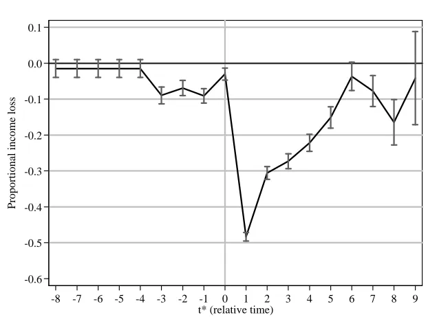
In Figure 1 we plot estimates of the income loss from the raw data without imposing any of the sample restrictions defined in Table 2. We constrain the␦kto
be equal in the reference periodⳮ8ⱕt*ⱕⳮ4 to obtain more accurate estimates of
the permanent difference in income between the groups. The treatment group has a slightly lower average wage in the predisplacement reference period untilt*ⳮ4, but
this is not significantly different from zero. Incomes of the treatment group then fall relative to the control group for ⳮ3ⱕt*ⱕⳮ1. However, immediately before
dis-placement att*⳱0 income losses become smaller. This is because, in the raw data, the treatment and control groups have different employment patterns in the predis-placement period. The treatment group has a higher incidence of nonemployment up tot*⳱ⳮ1, whereas att*⳱0 everyone in both treatment and control groups are
employed by definition (otherwise they could not be displaced). This illustrates why explicit matching of the treatment and control groups on the basis of predisplacement characteristics is important. Income losses from t*⳱1 onwards are large and
sig-nificant, in every year apart from t*⳱6 and t*⳱9 with a total loss of about 20 percent per year, which corresponds to a total loss of just under two years of in-work income.
A. Choice of estimation method
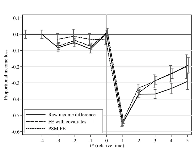
We now consider the effect of the estimation method on estimated income losses. In Figure 2 we plot estimates of␦k from Sample 1 from: (a) a simple raw
compar-ison;24 (b) a standard fixed-effects model; and (c) a fixed-effects regression on a sample of matched pairs constructed using propensity score matching.
The raw income loss is larger than the income loss estimated using the regression methods. For Sample 1, the fixed-effects regression and the propensity score method produce almost identical estimates of postdisplacement income losses. Total losses over the first five years after displacement are 32 percent per year.
-0.6 -0.5 -0.4 -0.3 -0.2 -0.1 0.0 0.1
Proportional income loss
-8 -7 -6 -5 -4 -3 -2 -1 0 1 2 3 4 5 6 7 8 9 t* (relative time)
Figure 1
Raw income losses, firm closure
The propensity score matching method also reduces the apparent predisplacement difference in income in period ⳮ3ⱕt*ⱕ0. The apparent reduction in the income loss at t*⳱0 observed in the raw data is removed by propensity score matching.
This is because we match exactly on predisplacement labour market history. As was noted, the predisplacement employment pattern of workers who are displaced is somewhat worse, which accounts for their lower predisplacement income in the raw data. The propensity score matching results suggest that the genuine predisplacement income effect is quite small (around 5 percent) and is only just significantly different from zero in the year immediately before displacement.
B. Choice of sample
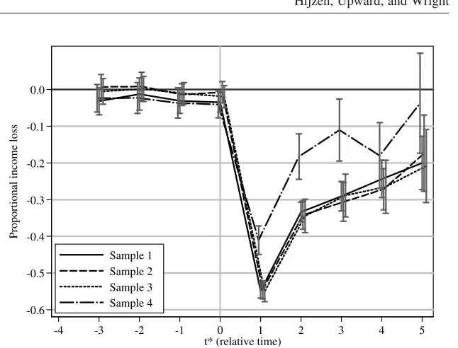
In Figure 3 we plot estimates of␦kusing propensity score matching for the different
samples described in Table 2. Samples 1, 2 and 3 provide very similar estimates of the cost of job loss once the predisplacement appearance pattern of workers is con-trolled for. As we would expect, Sample 2, which comprises workers employed in all four years before displacement, has larger income losses than sample 1, but the difference is not significant. Income losses for Sample 3, which excludes multiple displacements are also very similar.
-0.6 -0.5 -0.4 -0.3 -0.2 -0.1 0.0 0.1
Proportional income loss
-4 -3 -2 -1 0 1 2 3 4 5
t* (relative time) Raw income difference
FE with covariates PSM FE
Figure 2
Comparison of estimation methods, sample 1, firm closure
most importantly, Figure 3 shows that one would reach different conclusions about the longevity of income losses with Sample 4. Focusing on those workers who are reemployed byt*⳱5 reduces the sample size considerably, and therefore lowers the
precision of the estimates. Nevertheless, the results suggest that income losses have effectively disappeared by t*⳱5, whereas for those samples which include
non-employed workers there are still significant income losses of around 20 percent. This suggests that the pure wage losses are smaller than income losses which include spells of nonemployment.25We investigate this further in sub-section E.
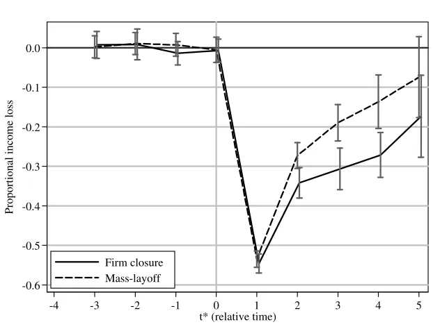
C. Choice of displacement definition
The next issue concerns the difference between the firm-closure sample and the mass-layoff sample. In Figure 4 we compare results from Sample 2 for the firm closure and mass-layoff definitions. For neither group is there any evidence of pre-displacement income losses. Losses immediately after layoff are very similar (within one standard error), but the mass-layoff sample has rather quicker recovery than the firm closure sample. This result is confirmed for all samples and for all estimation methods (see Tables 5 and 6).
-0.6 -0.5 -0.4 -0.3 -0.2 -0.1 0.0
Proportional income loss
-4 -3 -2 -1 0 1 2 3 4 5
t* (relative time) Sample 1
Sample 2 Sample 3 Sample 4
Figure 3
Comparison of samples, PSM FE estimates, firm closure
This result contrasts with Gibbons and Katz (1991). In their model layoffs are the result of firm discretion, which means that workers displaced in layoffs will tend to be of lower quality than those displaced by plant closures. If this is the case, post-displacement wages and incomes should belower for those displaced in mass lay-offs. There are two possible explanations for the difference between our results and those from the United States. First, our mass-layoff sample includes workers who exit the firm voluntarily. In contrast, Gibbons and Katz (1991) use self-reported displacement data from the DWS which excludes voluntary leavers. Second, differ-ent institutional features of the U.S. and U.K. labor market suggest that the selection of which workers to fire when plants make mass layoffs may be different. Mass layoffs in the United Kingdom are often accommodated by voluntary redundancies, and so selection effects would work in the opposite direction.26Those workers with less to lose will be the ones to leave companies which downsize. As far as we are aware, there is no direct evidence on this issue for the United Kingdom.
-0.6 -0.5 -0.4 -0.3 -0.2 -0.1 0.0
Proportional income loss
-4 -3 -2 -1 0 1 2 3 4 5
t* (relative time) Firm closure
Mass-layoff
Figure 4
Comparison of displacement definition, Sample 2, PSM FE estimates
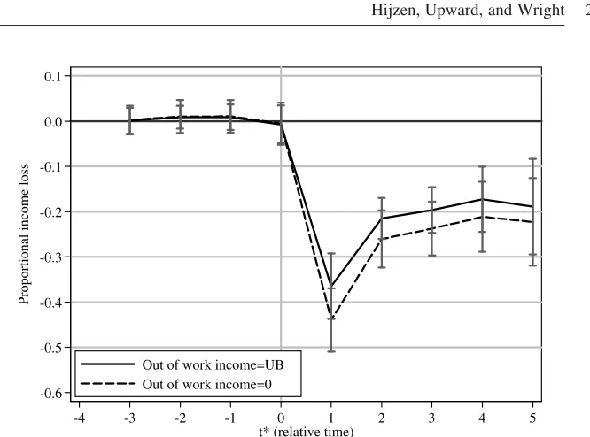
D. Definition of out-of-work income
The large income effects that we have observed are largely a result of spells of nonemployment, for which we impute income based on benefit levels. We have focused initially on these results as they allow us to examine the impact of displace-ment on workers’ wellbeing. However, JLS assume an income of zero for periods of nonemployment. To provide a closer comparison to the existing literature, Figure 5 compares the results obtained when out-of-work income is set equal to the benefit level and equal to zero. As would be expected, since the treatment group have a higher unemployment rate than the control group (after displacement), assuming zero out-of-work income increases the estimated loss. Since the unemployment differ-ential between the treatment and control group is 0.45, and the level of job-seekers allowance is approximately 11 percent of the mean in-work income, the loss att*⳱1
increases from 37 to 44 percent.
E. Pure wage effects
-0.6 -0.5 -0.4 -0.3 -0.2 -0.1 0.0 0.1
Proportional income loss
-4 -3 -2 -1 0 1 2 3 4 5
t* (relative time) Out of work income=UB
Out of work income=0
Figure 5
Comparison of out of work income definitions, Sample 2, PSM FE unlogged esti-mates
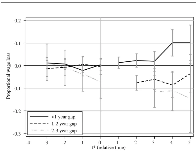
The treatment group is split according the length of time after displacement until the individual reappears in the data. Thus the solid line plots estimates of ␦k for
those who return to employment within 12 months of the displacement (for example, they are observed in the NES in the April after displacement). It is noticeable that, on reentry, wages are ranked exactly as we might expect: those with longer gaps have larger wage losses. However, even for those with some gap, wage losses are very small compared to the income losses observed in Figures 1 to 2. In addition, the relatively small sample size of the treatment group (especially when we split by the length of gap) means that these estimates are rather imprecise and confidence intervals overlap. Unfortunately, we cannot estimate wage effects beyond t*⳱5
without reducing the sample size ever further. It is therefore possible that wage losses continue to grow for those who have a longer gap after displacement.
F. Summary of results
In Tables 5, 6 and 7 we summarise all our results. We report the proportional cost per year for (a) all five years after displacement; (b) the first year after the displace-ment and (c) the fifth year after displacedisplace-ment.27
-0.3 -0.2 -0.1 0.0 0.1 0.2
Proportional wage loss
-4 -3 -2 -1 0 1 2 3 4 5
t* (relative time) <1 year gap
1-2 year gap 2-3 year gap
Figure 6
Wage loss estimates split by length of gap, Sample 5, FE estimates
As Figure 4 showed, estimated losses from the mass-layoff sample tend to be smaller than those from the firm closure sample, and also point to a faster recovery. Yearly losses over the first five years are in the range 18–35 percent for the firm closure sample, and 14–25 percent for the mass-layoff sample.
In every case the estimated losses diminish over time: losses five years after displacement are almost always a small fraction of losses one year after displace-ment. In the case of samples 4 and 5, estimated losses in year five are insignificantly different from zero, suggesting that the displaced catch up with the nondisplaced within five years. The crucial distinction is that samples 4 and 5 exclude individuals who do not reenter employment.
Sample 5 estimates are always the smallest because they ignore the income losses of workers who are not observed in the NES. Displaced workers who reappear in employment within 12 months have wage losses which are small and insignificantly different from zero in every case. In some cases these workers actually experience small wagegainscompared to the control group.
The final row of each panel of Tables 5 and 6 shows that therearewage losses, but only for workers who experience a “gap” (which we assume is a period of nonemployment) after displacement. Workers with a gap att*⳱1 have wages some
Hijzen,
a. Number reported is the cost per year as a proportion of the income of the control group at the same point in time.
b. Robust standard errors in parentheses; standard errors for matching estimators are bootstrapped (50 replications). *** significant at 1 percent; ** significant at 5 percent; * significant at 10 percent.
The
Summary of results: mass-layoff sample
DiD FE Matching, FE
a. Number reported is the cost per year as a proportion of the income of the control group at the same point in time.
b. Robust standard errors in parentheses; standard errors for matching estimators are bootstrapped (50 replications). *** significant at 1 percent; ** significant at 5 percent; * significant at 10 percent.
Table 7
Comparison of zero and nonzero out of work income: closure sample
Nonzero out of work
Notes: Number reported is the cost per year as a proportion of the income of the control group at the same point in time. Bootstrapped standard errors in parentheses. All estimates are estimated using Equation 1 on propensity score-matched treatment and control groups.
losses which include periods of nonemployment. In contrast to JLS therefore, we find less evidence that income losses are driven by wage losses. Instead, income losses are driven by spells of nonemployment.
The results presented in Tables 5 and 6 assume that out-of-work income is set at the level of jobseekers’ allowance. However, the majority of previous studies, es-pecially those from the United States, examine labour earnings loss. When a person is unemployed their labour earnings are, by definition, zero. In order to aid com-parability with previous work, Table 7 presents, for each of our samples, the income losses from firm closure when out-of-work income is set equal to zero.28
Since in these estimations out-of-work income is now zero, the dependent variable is unlogged. In order to isolate the pure effect of assuming zero out-of-work income,
abstracting from the change in functional form, Column 1 in Table 7 also reports the unlogged results when assuming nonzero out-of-work income. Column 1 is sim-ply therefore the unlogged version of Column 3 of Table 5. As before however, the results of these estimations are presented as percentage losses so that the results are directly comparable across tables. The use of zero out-of-work income will increase the estimated losses if the treatment group has higher post-displacement unemploy-ment rates than the control group. As would be expected, this is always true, on average, for the first five years after displacement for Samples 1–4. For example, the loss for Sample 2 over the first five years is 23 percent if we include out-of-work income, and this increases to 27 percent if we set out-of-out-of-work income to zero. The increase in the estimated loss is between 1 (Sample 4) and 5 (Sample 1) per-centage points. This relatively small impact reflects the low replacement ratios of U.K. benefits. The treatment group has higher relative unemployment rates imme-diately after displacement and so the estimated loss increases by more att*⳱1 than
att*⳱5. Note that the modelling decision has no impact on sample 5, because here
the sample is restricted to those in employment in all periods after displacement.
Heterogeneity of displacement costs
Much of the previous literature has emphasised that losses are likely to vary sub-stantially across individuals. In this section we report estimates for various subgroups of the data. In each case we use sample 2 and report fixed-effects estimates of Equation 1 using matched treatment and control groups. The results are reported in Table 8.
An interesting issue, and an important difference between our sample and that of JLS, is that we use a random sample of all displaced workers, whereas they restrict the sample to those workers with at least six or more years of tenure in 1980. This could potentially lead to higher estimates of losses on their part. Although our data does not contain a direct measure of tenure, the NES records whether an individual is in the same “position” as 12 months earlier.29
Using this measure we can split the sample according to whether a worker has more or less than four years in the same position within the firm at the time of displacement. As expected, losses are much greater for those with higher tenure. Five years after displacement the losses of short-tenure workers are insignificantly different from zero. Long-tenured workers have losses of more than 25 percent. This is actually close to JLS’s estimate of long-term losses. However, we still find that this loss is primarily due to employment rather than wage differences, because es-timated losses for high tenure workers from Sample 4 are only 7.1 percent after five years, and insignificantly different from zero.30Thus, even for high tenure workers we do not find significant wage losses in the long-run.
29. Using this variable will therefore underestimate tenure within the firm, since within firm changes will count as a change of position. In addition, because this is a cumulative measure, it is not possible to measure the actual length of long spells of tenure at the beginning of the sample period.
Table 8
a. Number reported is the cost per year as a proportion of the income of the control group at the same point in time.
b. Bootstrapped standard errors in parentheses.
We find that losses are larger for older workers. Over all five years, older workers lose about 39 percent of their predisplacement income per year, compared to 32 percent for younger workers.
The next panel shows that men experience significantly larger losses than women: 40 percent per year compared to 29 percent. This difference is sustained up to and including the fifth year after displacement. These results are consistent with those for the United States from JLS, and might be explained by the different occupations and industries which men work in. For example, the losses associated with displace-ments from manufacturing industries are somewhat larger than those from the service sector.
We also split the sample according to individuals’ occupation att*⳱0.31We find that initial losses are larger for skilled workers, which is consistent with the notion that firm-specific human capital is an important component of skilled workers’ wages. Byt*⳱5 losses are slightly smaller for skilled workers, although fromt*⳱2
onwards estimates for the two groups are insignificantly different from each other.
VI. Conclusions
We have examined the income losses of displaced workers using a new matched worker-firm dataset for the United Kingdom. Our estimates suggest that the costs during the first five years after the displacement event are in the range 18–35 percent per year for workers whose firm closes down, and 14–25 percent for workers who exit a firm which suffers a mass layoff. If we exclude out-of-work income, these losses increase by approximately 4–5 percent per year.
Income losses are rather less heterogeneous than in the United States, although the size of the loss varies in predictable ways. Those workers who are older, male, working in manufacturing, skilled and with higher seniority lose more. These costs are substantially a result of periods of nonemployment. This contrasts with the well-known results of Jacobson et al. (1993), who find large income losses are not caused by greater rates of nonemployment.
We have shown that results are sensitive to the choice of control and treatment groups, and the definition of displacement. The U.S. literature tends to focus on “high tenure” workers, and uses a control group which remains in employment in the same firm throughout. As an estimate of theaveragecost of a lost job, we feel that this is not an appropriate comparison. When a firm closes down, both high- and low-tenure workers are affected. Also, workers who are not displaced still face a risk of job loss in the future, albeit smaller than those who are displaced.
The choice of sample and comparison group also crucially affects the conclusion one draws about the “permanence” of income loss. We find little evidence for per-manent income losses for workers who return to employment, but large losses (up
to 20 percent of the predisplacement income) when we include workers who remain out of the sample.
Our results are consistent with the European findings reported in Kuhn (2002), which show small wage losses, which is in itself consistent with the conventional wisdom that wages are more flexible in the United States, and that transitions into work are slower in the United Kingdom and Europe. Although our results are sug-gestive, we do not think that the existing micro-level evidence is sufficient to con-fidently state that the smaller wage losses observed in the United Kingdom are the result of a specific labour market institution such as longer benefit duration. As Addison and Blackburn (2000) note, “There is surprisingly little research into the effects of unemployment insurance (UI) on post-unemployment wage outcomes.”32 This would be an interesting area for future research.
Our results do not necessarily imply that policy-makers should seek to protect jobs. Indeed, there has been a growing awareness in the policy-making community that, due to ongoing globalization and technological change, flexibility for firms to respond to changes in market conditions is increasingly important. Instead of con-centrating on protecting jobs it may be more fruitful for governments to focus di-rectly on the needs of workers. The analysis in the present paper of the nature of displacement costs in the United Kingdom provides a number of useful insights in this regard. First, the sheer size of the income losses suggests that direct adjustment assistance to displaced workers is bound to be an important ingredient of any com-prehensive policy package. Second, the finding that the bulk of displacement costs represents unemployment spells and not wage losses upon reemployment, as is gen-erally found to be the case in the United States, suggests that governments should primarily focus on ways to promote employment. Direct adjustment assistance and pro-employment policies do not have to be inconsistent as long as financial support to displaced workers is not excessive, is accompanied with training and jobseeker services, and is conditional on search effort. A comprehensive policy framework such as that presented in the restated OECD Job Strategy (OECD 2006) provides a useful starting point.
References
Abbring, Jaap H., Gerard J. van den Berg, Pieter A. Gautier, A. Gijsbert C. van Lomwel, Jan C. van Ours, and Christopher J. Ruhm. 2002. “Displaced Workers in the United States and the Netherlands. InLosing Work, Moving on: International Perspectives on Worker Displacement,ed. Peter Joseph Kuhn. Kalamazoo, Mich.: W.E. Upjohn Institute. Addison, John T., and McKinley L. Blackburn. 2000. “The Effects of Unemployment
Insur-ance on Post Unemployment Earnings.”Labour Economics7(1):21–53.
Addison, John T., and Pedro Portugal. 1989. “Job Displacement, Relative Wage Changes, and Duration of Unemployment.”Journal of Labor Economics7(3):281–302.
Arulampalam, Wiji. 2001. “Is Unemployment Really Scarring? Effects of Unemployment Experiences on Wages.”Economic Journal111(475):F585–606.
Ashenfelter, Orley C. 1978. “Estimating the Effect of Training Programs on Earnings.” Re-view of Economics and Statistics60(1):47–57.
Bender, Stefan, Christian Dustmann, David Margolis, and Costas Meghir. 2002. “Worker Displacement in France and Germany.” InLosing Work, Moving on: International Per-spectives on Worker Displacement,Chapter 5: 375–470. ed. Peter Joseph Kuhn, W.E. Upjohn Institute.
Blundell, Richard, and Monica Costa Dias. 2002. “Alternative Approaches to Evaluation in Empirical Microeconomics.” CeMMAP Working Papers CWP10/02, Centre for Microdata Methods and Practice, Institute for Fiscal Studies, October.
Booth, Alison. 1987. “Extra-statutory Redundancy Payments in Britain.”British Journal of Industrial Relations25(3):401–418.
Borland, Jeff, Paul Gregg, Genevieve Knight, and Jonathan Wadsworth. 2002. “They Get Knocked Down, Do They Get Up Again? Displaced Workers in Britain and Australia.” InLosing Work, Moving on: International Perspectives on Worker Displacement,ed. Pe-ter Joseph Kuhn, ChapPe-ter 4, 301–76. W.E. Upjohn Institute.
Burda, Michael C., and Antje Mertens. 2001. “Estimating Wage Losses of Displaced Work-ers in Germany.”Labour Economics8(1):15–41.
Cameron, A. Colin, and Pravin K. Trivedi. 2005.Microeconometrics: Methods and Applica-tions. Cambridge.
Carrington, William J. 1993. “Wage Losses for Displaced Workers: Is It Really the Firm That Matters?”Journal of Human Resources28(3):435–62.
Eliason, Marcus, and Donald Storrie. 2006. “Lasting or Latent Scars? Swedish Evidence on the Long-term Effects of Job Displacement.”Journal of Labor Economics24(4):831–56. Farber, Henry. 2003. “Job Loss in the United States, 1981–2001.” NBER Working Papers
9707, National Bureau of Economic Research, May.
Gibbons, Robert, and Lawrence F. Katz. 1991. “Layoffs and Lemons.”Journal of Labor Economics9(4):351–80.
Gregory, Mary, and Robert Jukes. 2001. “Unemployment and Subsequent Earnings: Esti-mating Scarring Among British Men 1984–94.”Economic Journal111(475):F607–25. Heckman, James J., Hidehiko Ichimura, and Petra Todd. 1998. “Matching As An
Econo-metric Evaluation Estimator.”Review of Economic Studies65(2):261–94.
Hildreth, Andrew K. G., Till M. von Wachter, and Elizabeth Weber Handwerker. 2005. “Estimating the ‘True’ Cost of Job Loss: Evidence Using Matched Data from California 1991–2000.” University of California-Berkeley, May. Unpublished.
Huttunen, Kristiina, Jarle Møen, and Kjell G. Salvanes. 2006. “How Destructive Is Creative Destruction? The Costs of Worker Displacement.” IZA Discussion Papers 2316, Institute for the Study of Labor (IZA), September.
Ichino, Andrea, Guido Schwerdt, Rudolf Winter-Ebmer, and Josef Zweimu¨ller. 2007. “Too Old To Work, Too Young To Retire?” IZA Discussion Papers 3110, Institute for the Study of Labor (IZA), October.
Jacobson, Louis S., Robert J. LaLonde, and Daniel G. Sullivan. 1993. “Earnings Losses of Displaced Workers.”American Economic Review,83(4):685–709.
Jones, Gareth. 2000. “The Development of the Annual Business Inquiry.”Economic Trends, (564):49–57.
Kletzer, Lori Gladstein. 1989. “Returns To Seniority After Permanent Job Loss.”American Economic Review,79(3):536–43.
——— 1996. “The Role Of Sector-specific Skills In Post-displacement Earnings.”Industrial Relations35:473–90.
Kuhn, Peter Joseph, ed. 2002.Losing Work, Moving on: International Perspectives on Worker Displacement. Kalamazoo, Mich.: W.E. Upjohn Institute.
Neal, Derek. 1995. “Industry-specific Human Capital: Evidence From Displaced Workers.” Journal of Labor Economics13(4):653–77.
Nickell, Stephen, Patricia Jones, and Glenda Quintini. 2002. “A Picture Of Job Insecurity Facing British Men.”Economic Journal112(476):1–27.
OECD. 2005. “Trade-adjustment Costs In OECD Labour Markets: A Mountain Or A Mole-hill?” InOECD Employment Outlook: 23–72. Paris: OECD.
——— 2006.Employment Outlook. Paris: OECD.
Office for National Statistics. 2001. “Review of the Inter-Departmental Business Register.” Office for National Statistics Quality Review Series No. 2.
Pfann, Gerard A., and Daniel S. Hamermesh. 2001. “Two-sided Learning, Labor Turnover, and Displacement.” NBER Working Papers 8273, National Bureau of Economic Re-search, May.
Podgursky, Michael, and Paul Swaim. 1987. “Job Displacement and Earnings Loss: Evi-dence from The Displaced Worker Survey.”Industrial and Labor Relations Review 41(1):17–29.
Rosenbaum, Paul R., and Donald B. Rubin. 1983. “The Central Role of the Propensity Score In Observational Studies For Causal Effects.”Biometrika70(1):41–55. Ruhm, Christopher J. 1991. “Are Workers Permanently Scarred By Job Displacements?
American Economic Review81(1):319–24.
Schoeni, Robert F., and Michael Dardia. 1997. “Earnings Losses of Displaced Workers in the 1990s.” JCPR Working Papers 8, Northwestern University/University of Chicago Joint Center for Poverty Research, July.
StataCorp. 2005.Stata Statistical Software: Release 9 Reference Manual R-Z. College Sta-tion, Tex.: Stata Corporation.
Stevens, Ann Huff. 1997. “Persistent Effects of Job Displacement: The Importance of Mul-tiple Job Losses.”Journal of Labor Economics,15(1):165–88.
Stevens, David W., Robert L. Crosslin, and Julia Lane. 1994. “The Measurement and Inter-pretation of Employment Displacement.”Applied Economics26(6):603–08.
Topel, Robert H. 1990. “Specific Capital and Unemployment: Measuring the Costs and Consequences of Job Loss.” Carnegie-Rochester Conference Series on Public Policy 33, 181–214.