Is there a Causal Effect of High School
Math on Labor Market Outcomes?
Juanna Schrøter Joensen
Helena Skyt Nielsen
a b s t r a c t
In this paper, we exploit a high school pilot scheme to identify the causal effect of advanced high school math on labor market outcomes. The pilot scheme reduced the costs of choosing advanced math because it allowed for a more flexible combination of math with other courses. We find clear evidence of a causal relationship between math and earnings for students who are induced to choose math after being exposed to the pilot scheme. The effect partly stems from the fact that these students end up with a higher education.
I. Introduction
Increased globalization has resulted in an increased focus on the ef-ficiency of education systems and the accumulation of high-quality skills—such as math skills—in high-wage countries. As a result, there is much public discussion about the optimal curriculum in many countries around the world. This paper is de-voted to the study of the effect of math, which is a core element of all curricula in primary and secondary schools.
It is well established that individuals with advanced math qualifications perform better on a range of important economic performance measures. High school gradu-ates with advanced math qualifications have higher test scores, attain a higher education, Juanna Schrøter Joensen is an assistant professor of economics at the Stockholm School of Economics. Helena Skyt Nielsen is a professor of economics and management University of Aarhus. The authors gratefully acknowledge financial support from the Danish Research Agency. They appreciate useful comments from Joshua Angrist, Nabanita Datta Gupta, Marianne Simonsen, Lars Skipper, Michael Svarer, Christopher Taber, as well as from discussants and participants at the DGPE, CEPR/IFAU/ Uppsala University, CEPR/EENEE/University of Padova, and ‘‘Do Schools Matter?’’ Aarhus School of Business workshops, the SMYE 2006 and ESPE 2006 conferences. The authors also would like to thank seminar participants at the University of Texas, the University of Aarhus, and Umea˚ University for comments on earlier drafts. The usual disclaimer applies. The data used in this article can be obtained beginning March 2010 through to February 2013 from Helena Skyt Nielsen, School of Economics and Management, University of Aarhus, Universitetsparken, Building 1322, DK-8000 Aarhus C, hnielsen@econ.au.dk. Data security policy means that access can be obtained from Aarhus only.
½Submitted September 2006; accepted September 2007
ISSN 022-166X E-ISSN 1548-8004Ó2009 by the Board of Regents of the University of Wisconsin System
and earn a higher income than those without.1The question is, however, to what ex-tent these observations indicate a causal impact of math on performance, and to what extent it is a selection effect indicating that people with other favorable characteris-tics choose to acquire higher math qualifications.
As a basis for policy discussion on changing high school curricula, hard evidence on the existence of the causal impact of math courses on labor market success is nec-essary. Policy recommendations are distinctly different depending on the conclusion. If we cannot reject the causal impact of math on outcomes relative to other subjects, the implication is that policy makers should consider an enhanced emphasis on math in high school curricula for all students. On the other hand, a rejection of the causal effect also dismisses the need for an enhanced math curriculum since it may lead to a potentially inefficient allocation of students and workers after high school.
In order to estimate the causal effect of math on earnings, a seminal paper by Altonji (1995) and its successors apply the curriculum of the average student from the high school in question as an instrument for acquired math qualifications. This instrument, however, is potentially invalid because the instrument is likely to be cor-related with unobservables that reflect earnings. In this paper, we instead suggest us-ing an instrument based on a Danish high school pilot scheme.
The pilot program was introduced prior to the comprehensive structural high school reform of 1988. The program was implemented prior to the reform as an ex-perimental curriculum at some high schools from 1984–87. Without the pilot scheme, advanced math was only offered in tandem with advanced physics, which scared away a lot of students potentially interested in math. Some high schools received an exemption and were allowed to test a pilot scheme in which advanced math could be combined with chemistry, which meant that about one-third more students chose advanced math among those unexpectedly exposed to the pilot scheme.
The information we use is on the population of high school students from the cohorts 1984–87, which is available in a brand new register-based data set. We have information about detailed educational event histories and about individual labor market histories, including actual labor market experience, degree of unemployment, and income. The data set is augmented with information about parents, courses taken in high school, and high school grade point averages (GPA).
Our empirical investigation of the effect of high school math on labor market out-comes confirms the finding of Rose and Betts (2004) that math matters. However, Rose and Betts (2004) stress that it is not entirely clear whether their estimates reflect selection or causality, whereas we claim that we get close to an estimate of a causal effect due to the availability of a strong and valid instrument. We find that students who choose the advanced math course earn roughly 30 percent more than other high school graduates and that the dominant part of this earnings premium reflects a causal impact. We estimate a causal effect for the subgroup of the population induced to choose advanced math because they unexpectedly were exposed to a pilot scheme allowing them to combine advanced math with advanced chemistry instead of phys-ics. As a consequence, the causal effect should be interpreted as the combined effect of taking advanced math and advanced chemistry.
The remainder of this paper is structured as follows: Section II surveys previous literature, while Section III describes the pre-1988 high school and the pilot scheme, which is central to the identification strategy of this paper. Next, Section V describes the data; Section V shows the results of the empirical analyses and, finally, Section VI concludes the paper.
II. Previous Studies
A causal effect of math on earnings may work through several chan-nels: enhanced cognitive or noncognitive skills, changed preferences for higher ed-ucation or enhanced productivity in completing a higher eded-ucation. In this study we focus on the still unresolved issue of whether the causal effect is significantly larger than zero or not, rather than the specific reasons for the effect.
Cross-country studies investigate the impact of math on economic performance. Both Hanushek and Kimko (2000) and the more convincing followup study by Jamison, Jamison, and Hanushek (2007), which uses a broader and longer data set, are con-cerned with the potential influence of the quality of education as measured by com-parative math and science test scores on growth. They find that one standard deviation increase in the math test score leads to an increase in annual growth rates of 0.5–1.0 percentage points, which only makes sense if there are strong externalities related to accumulating high-quality human capital. Hence, cross-country studies in-dicate that there is a positive effect from high-quality math skills on economic growth, which they claim is causal. In line with a handful of earlier papers, we com-plement these studies by confronting their hypothesis with individual data.
A number of papers have studied the effect of high school curricula on individual earnings. Altonji (1995) pioneered this area of research. In a study based on the Na-tional Longitudinal Study of the High School Class of 1972 (NLS72), he uses the variation in curricula across U.S. high schools to identify the effects of coursework on wages and educational outcomes. He finds a negligible effect from specific cour-sework, including math. Altonji (1995) uses the curriculum of the average student from the high school in question as an instrument for the math qualifications ac-quired. However, as he points out, this experiment is not a clean natural experiment because the curriculum of the average individual at a given high school may be cor-related with the average family background, primary school preparation, ability of the student body, and the quality of the courses. However, Altonji (1995) argues that the potential bias is positive, which means that the small effect of specific course-work that he finds may be interpreted as an upper bound. As an alternative, he tries to control for high school specific effects by including school-level observed varia-bles and by including high school fixed effects (FE), which gives small curriculum effects that are slightly higher than the effects estimated by IV.
Levine and Zimmerman (1995) use a similar approach. They find slightly stronger effects when comparing the results of analyses based on the National Longitudinal Study of Youth (NLSY) with analyses of the 1980 cohort from High School and Be-yond (HSB). However, any potential effects are still restricted to certain subgroups (men with a low education and highly educated women), which raises doubt about the existence of the causal impact of coursework on labor market outcomes.
Rose and Betts (2004) use data for the 1982 cohort from HSB, which is an im-mense improvement upon earlier studies for several reasons. First of all, the tran-script data for the sampled individuals are more detailed than those used in the earlier papers. Second, the individuals are observed when in their thirties rather than in their twenties, and finally, the individuals are observed after the huge increase in college premiums around 1990. Rose and Betts (2004) find that math matters. They disaggregate math into six courses, and estimate the return on each of the six math courses compared to the average curriculum. They perform a whole battery of ro-bustness checks using OLS, Altonji’s IV, and school fixed effects. The most robust conclusion across all the tests is that course credits in algebra/geometry significantly increase earnings.
As the authors themselves are aware, it is unclear whether the results of the pvious studies (Altonji 1995; Levine and Zimmerman 1995; Rose and Betts 2004) re-flect selection or causality. Our study improves upon these studies by getting closer to the causal impact of math while applying a better instrument for acquired math qualifications. We use an instrument based on a pilot scheme implemented for the cohorts starting in the Danish high school before the structural reform of 1988. In the following subsection we describe the context of this pilot program.
III. Pre-1988 High Schools and the
Pilot Program
From 1961 through 2005, a central distinction has been made in the Danish high schools2 between educations centered on mathematics (‘‘math track’’) and on language studies (‘‘language track’’). Our focus is on the ‘‘branch-based’’ high school system that existed from 1961 to 1988, where courses were grouped in restrictive course packages. We focus on this period for two reasons: First, the sup-ply of course packages provides us with exogenous variation in the cost of acquiring advanced math qualifications due to the gradual introduction of a pilot program. Sec-ond, the focus on individuals attending high school in the pre-1988 system means that our data set includes labor market outcomes for the individuals when they are in their thirties.
In this section we describe aspects of the relevant high school system first, includ-ing the pilot program. Then, we describe the construction of an instrumental variable based on the pilot program.
A. Math in pre-1988 high schools
were available for the math track students was: ‘‘to teach them a number of mathe-matical concepts and ways of thinking, to prompt their sense of clarity in expressions and logical inference in proofs, to enhance their imagination and ingenuity, to let them practice handling case studies (including execution of numerical arithmetic), and to provide familiarity with applications of mathematics within other fields.’’3 The objective of the low-level math course for language track students was partly to provide them with an introduction of the mathematical methods and partly to give them some mathematical tools that could be useful to them later.
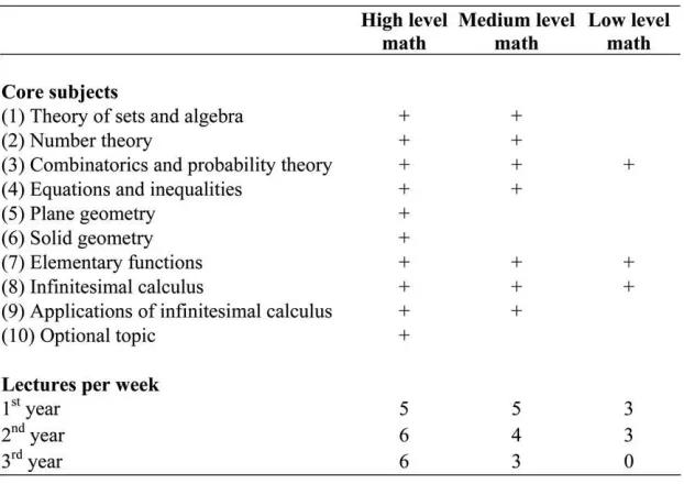
In Figure 1, we summarize the contents of the three types of math courses avail-able. The main difference between the high-level and the intermediate-level math is that geometry (Core Subjects 5 and 6) is not taught in the intermediate-level course. Furthermore, some subjects were treated differently when taught at the intermediate course level compared to the high-level course. In the low-level math course, the content was reduced to elementary functions, combinatorics and probability theory, and infinitesimal calculus.4
In the empirical analysis, we distinguish between whether individuals take the high-level math course, which means intermediate- and low-high-level courses are lumped to-gether, providing a binary indicator for choosing high-level math (MathA). In addition Figure 1
Overview of the Content of Math Courses
3. Quotation from the high school mission statement, see Petersen and Vagner (2003). 4. See Petersen and Vagner (2003) for further details on the math curricula.
to the number of lessons, the main difference between the high-level and the inter-mediate-level math course is geometry. According to Rose and Betts (2004), algebra and geometry are the mathematical subjects that most reliably give a consistently positive effect on future earnings. Therefore, if there is a causal effect of math, we expect it to show up in this set-up.
B. Structure of pre-1988 high schools
The high schools attended by the pre-1988 cohorts were structured as follows: Upon entry, the students chose between the math track and the language track. After the first year, they chose one of the eight branches that are summarized in Figure 2: Figure 2
socsci-languages, music-languages, modern languages, classical languages, math-socsci, math-natsci, math-music, or math-physics. Students enrolled at a pilot school also had the option to choose the math-chemistry branch. Language track students could choose between the first four course packages, while math track students could choose between the last four branches (or five, if they were at a pilot school).
As is evident from Figure 2, the only way to obtain the high-level math course was to opt for the math-physics branch, unless you were enrolled at one of the pilot schools that offered the math-chemistry branch. The increased course flexibility at the pilot schools gave students an added incentive to choose high-level math since the students were not necessarily compelled to choose high-level physics, which is considered a tough course.5
C. Pilot program in pre-1988 high schools
The pilot scheme was implemented as an experimental curriculum at some high schools prior to the 1988-reform. Table 1 gives an overview of the gradual imple-mentation of the pilot scheme from 1984–87. The table is divided by types of high schools: schools with no pilot scheme (PilotSchool¼0), schools where the pilot scheme was introduced after enrollment of the relevant cohort (PilotSchool¼1 & PilotIntro¼1), and schools where the pilot scheme was implemented prior to enroll-ment of the relevant cohort (PilotSchool¼1 & PilotIntro¼0). Furthermore, the table lists the percentage choosing high-level math for each cohort in each school type (MathA¼1). The pilot scheme allowed for a more flexible combination of advanced math with other high school courses, which meant that about one-third more students among those who unexpectedly were exposed to the pilot scheme chose advanced math.
Schools were not randomly assigned to become pilot schools. Instead, from 1984– 86, they could apply to the Ministry of Education for permission to adopt the exper-imental curriculum, whereas in 1987, the high school principals could make this decision without approval from the ministry. From 1984–87 roughly 50 percent of the high schools adopted the experimental curriculum, and those schools were evenly spread geographically. It is not possible to check whether the pilot schools represent a sample of schools which is essentially random with respect to math ability.
Individuals attend high school by applying to the ones they would prefer to attend. If admission is not granted by the school preferred, the application is subsequently sent to the applicants’ second priority. All students who have completed nine years of compulsory schooling may be admitted either directly or after passing an entry exam. All qualified applicants are guaranteed admission to a school in the county they live in.
If schools currently offered the math-chemistry branch, this would be advertised in the marketing material, allowing students to take this into account when they filled out their applications. In their application letters, students could indicate that they
5. Albæk (2003) backs up this conclusion with a simple theoretical model in which he analyzes the effect of restricted course packages on the choice of high school courses in a framework where the student max-imizes his or her future probability of being accepted at a university, which is assumed to be based on GPA. This approach is consistent with the Danish postsecondary schooling system that screens students based on their GPA and which courses they took in high school.
Table 1
Overview of the Introduction of the Pilot Scheme in Danish High Schools
Year
1984 121 11,871 24.8 22 3,005 32.5 0 0 143 14,876 26.4
1985 105 9,894 23.7 15 1,615 35.0 22 2,774 33.9 142 14,283 27.0
1986 90 7,825 21.7 15 1,512 33.3 37 4,224 37.0 142 13,561 27.8
1987 77 7,207 20.0 12 1,349 28.5 52 6,360 35.2 141 14,916 27.2
Total 36,797 22.9 7,481 32.5 13,358 35.5 57,636 27.1
Note: This table, which explains how the pilot scheme was introduced in high schools from 1984–87, shows the number of high schools and the corresponding amount of students by entry cohort. The table is divided by types of high schools: schools with no pilot scheme (PilotSchool¼0), schools where the pilot scheme was introduced after enrollment of the relevant cohort (PilotSchool¼1, PilotIntro¼1), and schools where the pilot scheme was implemented prior to enrollment of the relevant cohort (PilotSchool¼1,PilotIntro¼0).
The
Journal
of
Human
preferred a given school due to the advertised option of choosing the math-chemistry combination after the first year. For the very first cohort exposed to the introduction of the math-chemistry combination at a given school, however, no advertising took place prior to making enrollment decisions, which means that the availability of the additional course combination could not have affected where students attended schools.
Table 2 compares the characteristics of the student body at pilot schools with the student body at nonpilot schools. We distinguish between students at pilot schools where the pilot scheme was unexpectedly introduced after they had enrolled in the high school (PilotSchool¼1 & PilotIntro¼1), and those who knew that the school was a pilot school before they applied (PilotSchool¼1 & PilotIntro¼0). The table reveals that the parental background of students who were unexpectedly exposed to the pilot scheme is less favorable than that of students at nonpilot schools (Column 2) and less favorable than that of students who were expectedly exposed to the re-form (Column 3). This is true both for the parents’ income and their education. Therefore, if anything, it seems that the schools that chose to implement the pilot scheme had a negatively selected sample of students rather than the opposite.
In the empirical analysis, we define an instrument that exploits the fact that some students were unexpectedly exposed to the pilot scheme. This instrument is described in the next subsection.
D. An instrumental variable based on the pilot program
The pilot scheme reduces the opportunity cost of choosing high-level math since the students exposed to the scheme are not required to take the physics course together with advanced math. Hence, first-year high school students enrolled at a school when it decided to introduce the pilot scheme were exposed to an exogenous cost shock. As documented in Table 1, this cost shock induces more students to choose high-level math compared to students at nonpilot schools. If the selection of newly participating schools is exogenous with respect to student ability, the pilot scheme may be seen as a natural experiment which provides exogenous variation in students’ math qualifi-cations without influencing the outcomes of interest other than through the effect on math qualifications. In the empirical analysis we account for the potential selec-tive participation of schools into the pilot program by adding controls that pick up qualifications of the local students; that is regional indicators and average character-istics of the student body at the school prior to 1984 when the pilot scheme started. The instrumental variable,PilotIntroi, is equal to one if the individuals enrolled in a high school which afterward decided to introduce the experimental curriculum for the first time and takes the value zero otherwise. This instrument isvalidif the pilot program is as good as randomly assigned to schools and if individuals are as good as randomly distributed across schools that have not yet decided to introduce the exper-imental curriculum. This assumption is violated only if the school decides to partic-ipate in the program based on the math ability of local students. The instrument is strongif the unexpected introduction of the scheme induces students to choose ad-vanced math, as Table 1 indicates that it does. The instrument satisfies the monoto-nicity condition if individuals who chose advanced math when it could only be combined with physics also would have chosen high-level math if they had unexpectedly
Table 2
Descriptive Statistics
Means and (standard deviations)
Variable Overall mean
Mean difference between PilotSchool¼1 PilotIntro¼1 and
PilotSchool¼0
Mean difference between PilotSchool¼1 PilotIntro¼1 and
PilotSchool¼1 PilotIntro¼0
Educational variables: High school:
Age at high school entry 16.24 (0.60) 0.00 0.03
Math track students 0.68 0.02 20.02
High level math 0.27 0.10 20.03
GPA 8.26 (0.97) 0.00 20.05
Highest completed education:
Length of education (years) 15.24 (2.37) 0.06 20.23
Educational level grouping:
High school only 0.17 20.01 0.01
Vocational training 0.11 0.01 0.03
Short higher education (SHE) 0.07 0.01 0.00
Medium higher education (MHE) 0.34 20.01 20.01
Long higher education (LHE) 0.27 0.02 20.03
Educational level-subject grouping:
High school only 0.17 20.01 0.01
Vocational training 0.11 0.01 0.03
SHE technical 0.02 0.00 0.00
The
Journal
of
Human
SHE other 0.05 0.00 0.00
MHE teacher 0.08 20.01 20.01
MHE humanities 0.04 0.00 0.00
MHE health 0.08 0.00 0.00
MHE socsci 0.05 0.00 0.00
MHE techsci 0.07 20.01 0.00
MHE other 0.02 0.00 0.00
LHE health 0.02 0.00 0.00
LHE natsci 0.03 0.00 20.01
LHE technical 0.06 0.01 0.00
LHE humanities 0.03 0.00 20.01
LHE socsci 0.10 0.01 20.01
LHE other 0.02 0.00 0.00
Other individual variables:
Log labor income (DKK) 12.12 (0.95) 0.02 20.03
Female 0.57 20.01 0.01
Labor market experience (years) 5.00 (2.71) 20.01 0.23
Parental background variables: Income:
FathersÕlog income (DKK) 9.05 (5.43) 20.03 20.17
MothersÕlog income (DKK) 8.41 (5.12) 20.21 20.29
Highest completed education:
Father elementary school only 0.16 20.01 0.02
Father high school 0.01 0.00 0.00
Father vocational training 0.28 0.01 0.01
Father short higher education 0.03 0.00 0.00
Father medium higher education 0.14 0.01 20.01
(continued)
Joensen
and
Nielsen
Table 2 (continued)
Means and (standard deviations)
Variable Overall mean
Mean difference between PilotSchool¼1 PilotIntro¼1 and
PilotSchool¼0
Mean difference between PilotSchool¼1 PilotIntro¼1 and
pilotSchool¼1 PilotIntro¼0
Father long higher education 0.11 20.01 20.02
Mother elementary school only 0.22 0.00 0.04
Mother high school 0.02 0.00 0.00
Mother vocational training 0.29 0.01 20.02
Mother short higher education 0.04 0.00 0.00
Mother medium higher education 0.17 20.01 20.02
Mother long higher education 0.04 0.00 20.01
Number of individuals 57,636
Note: This table shows descriptive statistics for the estimation sample consisting of high school graduates from the 1984–87 high school cohorts. For indicator variables the proportion of the sample included in the group is shown. For other variables the table provides the mean and the standard deviation (in parenthesis). Incomes are measured in 2000 prices. The exchange rate on Dec 31, 2000 was DKK 8.02 per USD. The first column of numbers shows the overall mean, the second column shows the differences between the characteristics of students who were unexpectedly exposed to the pilot scheme and students at nonpilot schools, while the third column shows the differences between the characteristics of students who were unexpectedly exposed to the pilot scheme and those expectedly exposed to the pilot scheme.
The
Journal
of
Human
had the option ofalsocombining it with advanced chemistry. We are confident that the monotonicity assumption is reasonable in our application since all the options available at nonpilot schools also were available at schools that introduced the pilot program.6
Our instrument exploits the exogenous variation in the exposure of students to the possibility of combining advanced math courses with advanced chemistry. Hence, the ‘‘treatment’’ that we investigate is the combined treatment of advanced math with advanced chemistry. Because advanced math and advanced chemistry are combined in a course package, we cannot separate the effect of advanced math from that of advanced chemistry or from the potential synergy effect of the combination of math with chemistry. However, the earlier literature suggests that if any specific course work matters, it is math rather than science courses that do so.7
Section IV identifies the effect of math on earnings for the compliers; that, is the group of students who were induced to choose math because they were allowed to combine advanced math with advanced chemistry rather than physics. The compliers are un-identifiable as they consist of a combined group of people who would otherwise have preferred to take an intermediate-level math course in combination with either ad-vanced social science, adad-vanced biology, or adad-vanced music courses (see Figure 3). Although unidentifiable, we find that the compliers are indeed a policy-relevant subgroup of students.8 Supplied with the option of choosing advanced chemistry, Figure 3
Distribution of Branch Choices, by PilotSchoolandPilotIntro
6. Consult Imbens and Angrist (1994) and Heckman, Lalonde, and Smith (1999) for details about the three IV assumptions.
7. See Altonji (1995), Levine and Zimmerman (1995), and Rose and Betts (2004). 8. See Heckman (1997).
the complying students end up with advanced math and advanced chemistry, poten-tially leading them to a different future career choice.
IV. Data
For our empirical analysis we use a brand-new rich panel data set comprising the population of individuals starting high school from 1984–87 in Den-mark. The data are administered by Statistics Denmark, which has gathered the data from different sources, but mainly from administrative registers, particularly for the purpose of this paper.
For each individual, we have data from complete detailed educational histories, including detailed codes for the type of education followed (level, subject, and edu-cational institution) and the dates for entering and exiting the education, along with an indication of whether the individual completed the education successfully, drop-ped out or is still enrolled as a student. Furthermore, we have information on the branch choice in high school and on high school GPAs.9The GPA is a weighted av-erage of final exam grades for each course. Both the quality of the courses and the GPA are comparable across high schools since monitoring high schools is centralized at the Ministry of Education. Furthermore, all high school students within each high school cohort take identical written exams, while oral exams and major written as-signments are evaluated both by the student’s own teacher and an external examiner assigned by the Ministry of Education.
Note that there are no tuition fees for education in Denmark, and all students 18 years and older receive a study grant from the government that suffices to cover liv-ing expenses.10Students living with their parents receive a reduced grant, but the grant is independent of parental income, educational effort, and achievement as long as the student is less than one year behind the prescribed norm.
We have yearly observations on labor income (earnings), gross income, and net income for 1997–2000. All incomes are observed at year-end and deflated to real val-ues measured in DKK in 2000 using the average wage index for the private sector. Other individual background variables used in our estimations are gender and actual labor market experience (including a squared term). The parental background varia-bles used include: A set of mutually exclusive indicator variavaria-bles for the level of highest completed education of the mother and father, respectively, and their income as observed at the end of the year before the individual started high school.
Among the gross population of high school entrants for 1984–87, only high school graduates who finished in three years are selected.11Furthermore, we exclude indi-viduals with missing labor market income 13 years after starting high school; hence,
9. In Denmark at that time a 13-point numerical grading scale system was used. The possible grades were 00, 03, 5, 6, 7, 8, 9, 10, 11, and 13; where 6 is the lowest passing grade, and 8 represents average perfor-mance.
10. Until 1996, the age limit was 19.
individuals who have left the country, died, are unemployed full-time year-round, or out of the labor force are excluded. Since students with high-level math are less likely to be unemployed or nonparticipants than others (see the next section), exclud-ing individuals with missexclud-ing incomes potentially introduces a negative bias on the parameter of main interest, meaning that our conclusion becomes conservative.12After the restrictions, the sample contains observations on 57,636 high school graduates, which makes about 14,000 graduates per cohort coming from about 140 different high schools, see Table 1.
A. Descriptive statistics
The descriptive statistics are shown in Tables 1–3. Table 1 gives an overview of the gradual implementation of the pilot program as well as the math choices of students at the high schools. Table 2 shows summary statistics of all background variables as well as the difference in these variables across school types, while Table 3 shows summary statistics of various outcome variables across school type as well as the dif-ferences by math level.
Table 1 shows that the proportion of the 1984 cohort that chose high-level math at the schools who unexpectedly provided the math-chemistry combination (PilotSchool¼1 & PilotIntro¼1) is 32.5 percent, whereas it is only 24.8 percent at the schools only offer-ing the math-physics combination (PilotSchool¼0). The proportion that chose high-level math at the nonpilot schools gradually declined from the 1984 cohort to the 1987 cohort, which indicates that students interested in math self-select into the high schools advertising that they offered the pilot scheme. On average, the difference in the proportion choosing high-level math at the schools unexpectedly offering the pi-lot program and the proportion choosing math at the nonpipi-lot schools is 10 percent-age points.
Tables 2 and 3 show that students who attended a pilot school have more favorable individual characteristics (apart from family background) than the students who attended nonpilot schools. The most favorable characteristics exist for students at schools who advertised their pilot status (PilotSchool¼1 & PilotIntro¼0), while the least favorable characteristics are found for individuals at nonpilot schools. Students who were unexpectedly exposed to the pilot scheme (PilotSchool¼1 & PilotIntro¼1) had 0.06 years more education and 2 percent higher earnings, on average, than the average graduate from a nonpilot school, while students who were expectedly ex-posed to the pilot scheme (PilotSchool¼1 & PilotIntro¼0) had an additional 0.23 years of education and an additional 3 percent higher earnings. The (raw) Wald es-timate of the effect of math on earnings is 0.2 (¼.02/.10) without controlling for any explanatory variables.
Table 3 reveals that the group of individuals choosing advanced math have more favorable characteristics no matter what the school type and that this group of stu-dents stands out even more at the nonpilot schools, where the stustu-dents are compelled to take advanced physics in order to take advanced math than they do at any of the
12. Our observations indicate 10 percent have missing labor income. They are distributed fairly equally across pilot and nonpilot schools and the estimation results are not sensitive to including these individuals with zero labor income.
Table 3
Descriptive Statistics of Labor Market and Educational Outcomes
Sample means and (standard deviations)
GPA in high school 8.26 0.24 8.25 0.25 8.29 0.23 8.24 0.20
(0.97) (0.97) (0.97) (0.96)
Sabbatical after high school:
Took sabbatical 0.82 20.11 0.79 20.18 0.81 20.13 0.84 20.11
Duration (years) of sabbatical after
0.84 0.07 0.83 0.08 0.87 0.05 0.83 0.05
Completed 1st attempted educ. successfully
0.61 0.09 0.60 0.10 0.63 0.08 0.60 0.08
Long Higher Educations:
Attempted long higher education 0.46 0.18 0.45 0.19 0.50 0.17 0.46 0.18
Completed long higher education 0.35 0.17 0.34 0.17 0.38 0.15 0.35 0.17
The
Journal
of
Human
Years from high school graduation until completion
8.62 21.08 8.71 21.12 8.40 20.97 8.59 21.01
(2.39) (2.44) (2.23) (2.43)
Length of highest completed education (years)
15.24 0.84 15.16 0.87 15.45 0.74 15.22 0.79
(2.34) (2.35) (2.32) (2.36)
Labor market outcomes:
Labor income (DKK) 12.12 0.30 12.10 0.31 12.15 0.29 12.12 0.26
(0.94) (0.95) (0.92) (0.95)
Degree of unemployment (scale 0–1000)
41.04 216.03 42.33 216.20 37.40 214.29 41.21 216.69
(124.97) (127.30) (118.35) (125.07)
Number of Individuals 57,636 36,797 13,358 7,481
This table shows descriptive statistics for the estimation sample consisting of high school graduates from the 1984–87 high school cohorts. For indicator variables the proportion of the sample included in the group is shown. For other variables the table provides the mean and the standard deviation (in parenthesis). Incomes are measured in 2000 prices. The exchange rate on Dec 31, 2000 was DKK 8.02 per USD.
Joensen
and
Nielsen
two school types offering the pilot program. High-level math students have higher high school GPAs and more high-level math students attend and complete a higher education at any level. Aside from having higher completion rates, high-level math students also complete a given educational level at a faster rate. Hence, high-level math students seem to be more efficient in the higher educational system. In addition, they are more successful after entering the labor market as they are unemployed less and earn more. High-level math students’ log earnings are 0.30 higher than the earn-ings of other high school students. As a point of reference, the math log earnearn-ings gap is more than five times larger than the gender log earnings gap for these high school graduates. Hence, we set out to find out whether this huge earnings gap is due to the fact that students become more productive on the labor market because they took the high-level math course or because the students with more favorable unobservable characteristics selected the high-level math course.
V. Results
In this section, we present our estimation strategy first, then we go through the main results, and, finally, we briefly present additional results as well as robustness tests. Let MathAi be an indicator for whether individual i chooses the high-level math course, and letYibe the log earnings of individuali. We estimate the following log earnings equation:
Yi¼b0+b1Xi+dMathAi+ei;
whereXiis a vector of characteristics of individuali. This vector includes individual characteristics, family background, cohort, and regional as well as school character-istics. Importantly, we always control for pilot school status,PilotSchooli, to allow for potential selection into pilot schools. The indicator variable for whether individ-ualichose the high-level math course in high school,MathAi, is potentially endog-enous since unobserved variables most likely exist affecting both earnings and the choice of high-level math. We assume that individuals chose high-level math if the expected gains exceeded the expected costs of the investment, that is ifYi1
The outcome variable, Yi, is (yearly) log earnings 13 years after starting high school. At that point in time, individuals, on average, have been on the labor market for about five years, and hence are likely to be settled into their careers. The preferred income measure would be lifetime income, which is impossible, however, to com-pute for our sample of individuals in their thirties.13
We use the Heckman two-step estimator to obtain consistent estimates of the causal effect of high-level math on earnings,d. Our main results estimate the total effect of math on earnings while leaving out postgraduation control variables. In this way, we give high school math credit for income increases that result from its effect on GPA, investments of time and money in higher education and labor market expe-rience. However, after the main part of the analysis at the end of this section, we briefly look at direct and indirect effects.
A. Main results
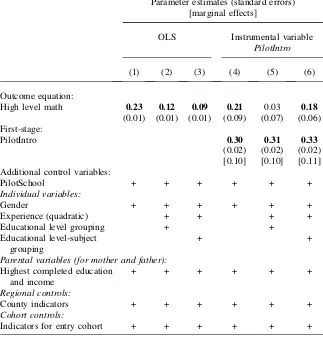
In Table 4, we present the estimates of the effect of math on earnings by OLS and IV.14 On the left hand side of the table, the results from OLS show that students who complete the high-level math course in high school receive 0.30 log points higher earnings on average. This number is reduced to 0.23 when we control for gen-der. Additional controls for parental background variables, region, cohort, and school indicators leave the parameter unchanged.
On the right hand side of the table, we present the results from IV estimation using the instrumentPilotIntroi. The IV estimates are generally smaller than the OLS esti-mates as would be expected in the event of a positive selection of students into the advanced math course. The IV estimate without explanatory variables other thanPilotSchoolishows a statistically insignificant effect of 0.16 of advanced math on earnings. This number increases to 0.28 and becomes significant when we control for gender. This indicates an interrelationship between gender and preference for the pilot scheme.15The standard high-level math course package, math-physics, seems to primarily appeal to boys, while the pilot program, math-chemistry, to a larger extent also appeals to girls. When we control for parental background variables, region, cohort, and school indicators, the effect of advanced math declines to 0.2.
This leads to the main conclusion of the paper, namely that the causal impact of math on earnings is significantly positive with a magnitude around 20 percent. This parameter should be interpreted as a local average treatment effect (LATE) identify-ing the effect for the subgroup of individuals who were induced to choose advanced math when they unexpectedly gained the opportunity to combine advanced math with advanced chemistry instead of advanced physics.16The estimated LATE param-eter may or may not be equivalent to the average treatment effect (ATE) or the average
13. The analysis has been done using three different income measures: gross income, net income, and labor market income. Furthermore, we have looked at income 12, 13, and 14 years after starting high school, respectively. Our qualitative results are robust to the change of income measure and year.
14. We also have estimated the model by using the instrument suggested by Altonji (1995), where the es-timated effect of math is then slightly larger than in the OLS.
15. Our data material does not allow for a separate analysis by gender. 16. See Imbens and Angrist (1994).
Table 4
Estimation of the Causal Effect of High Level Math on Labor Income for High School Graduates
Parameter estimates (standard errors) [marginal effects]
OLS Instrumental variablePilotIntro
(1) (2) (3) (4) (5) (6) (7) (8) (9) (10)
Outcome equation:
High level math 0.30 0.23 0.23 0.23 0.23 0.16 0.28 0.21 0.19 0.21 (0.01) (0.01) (0.01) (0.01) (0.01) (0.12) (0.09) (0.09) (0.10) (0.09) First-stage:
PilotIntro 0.29 0.31 0.30 0.16 0.28
(0.02) (0.02) (0.02) (0.03) (0.02) [0.10] [0.11] [0.10] [0.07] [0.10] Additional control variables:
PilotSchool + + + + + + + + + +
Individual variables:
Gender + + + + + + + +
Parental variables (for mother and father)
Highest completed education and income + + + + + + Regional controls:
County indicators + + + + + +
Cohort controls
Indicators for entry cohort + + + + + +
High school specific controls:
High school indicators + +
Average parental background in 1983 + +
Note: This table shows estimates of the effect of high level math on the log labor income thirteen years after starting high school. The two different estimation strategies are: Ordinary Least Squares (OLS) on the total sample of high school graduates from the 1984–87 high school cohorts and an Instrumental Variables (IV) estimation using
PilotIntroas an instrument. There are five distinct specifications for each estimation strategy, corresponding to Columns 1-5 and 6-10. They differ by the explanatory variables included andÔ+Õindicates which sets of explanatory variables are included in the estimation. The top row provides the parameter estimates of the effect ofMathA
on log labor income and the standard errors (in parentheses). The bottom row provides the parameter estimates regarding the instrument in the first-stageMathAselection equation, standard errors (in parentheses) and marginal effects [in square brackets]. Numbers written inboldindicate that the parameter is significant at the 1 percent level.
The
Journal
of
Human
treatment effect on the treated (ATET).17However, the LATE estimates the treatment effect of a policy-relevant subgroup of students.18The magnitude of the estimate is large and indicates that choosing the math-chemistry branch increases earnings by 20 percentrelative to the earnings of an average high school student without advanced math. Hence, if the rate of return for a year in high school is 8 percent, the rate of return may be for example 7.5 percent per year for an average student without ad-vanced math, while it would be 20 percent larger, that is 9 percent per year, for a student who was induced to choose advanced math when faced with the possibility of combining it with chemistry.
B. Additional results and tests
In this section, we present additional results as well as various tests of the robustness of our results and the validity of the pilot scheme based instruments. We use Spec-ification 8 from Table 4 as our benchmark case and add controls and perform tests treating this specification as our preferred specification.
1. Adding postgraduation controls
Our main results estimate the total effect of math on earnings where postgraduation control variables are left out. In this way, we give high school math credit for direct as well as indirect effects on income. In Table 5, we briefly present the results of es-timation after controlling for postgraduation controls in order to gain insight into the direct as well as indirect effects of math on earnings through educational choice and experience.
When we include measures of length of further education, the effect of math dis-appears (and goes from 0.21 to 0.03), which indicates that the effect of advanced math mainly goes through the increased probability of acquiring a higher education. Individuals who were induced to choose high-level math because they were unex-pectedly exposed to the experimental curriculum end up with longer educations than they otherwise would have gotten. We conclude that the main part of the causal effect of math on earnings is an indirect effect which goes through the effect on length of education. This effect may stem from changed preferences for length of education, or it may stem from improved skills for completing a longer education.19When we in-clude measures of the subject of further education, the effect of advanced math increases again to 0.18, which indicates that the compliers do not necessarily choose more favorable subjects of study.
2. Overidentification tests
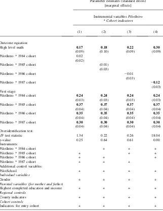
In Table 6, we exploit the fact that the pilot program was implemented gradually to tests for overidentification. We create four new instrumental variables which allow us
17. For discussion of treatment effect homogeneity, see Angrist (2004) and Heckman, Lalonde, and Smith (1999).
18. See Heckman (1997).
19. In a U.S. context, Arcidiacono (2004) finds that individuals with high math ability prefer the subjects and the jobs associated with lucrative majors.
Table 5
Estimation of the Causal Effect of High Level Math on Labor Income for High School Graduates Including Post-Graduation Variables
Parameter estimates (standard errors) [marginal effects]
OLS Instrumental variable
PilotIntro
(1) (2) (3) (4) (5) (6)
Outcome equation:
High level math 0.23 0.12 0.09 0.21 0.03 0.18
(0.01) (0.01) (0.01) (0.09) (0.07) (0.06) First-stage:
PilotIntro 0.30 0.31 0.33
(0.02) (0.02) (0.02) [0.10] [0.10] [0.11] Additional control variables:
PilotSchool + + + + + +
Individual variables:
Gender + + + + + +
Experience (quadratic) + + + +
Educational level grouping + +
Educational level-subject grouping
+ +
Parental variables (for mother and father): Highest completed education
and income
+ + + + + +
Regional controls:
County indicators + + + + + +
Cohort controls:
Indicators for entry cohort + + + + + +
to perform some tests of overidentification. Each new instrument is a cohort dummy interacted withPilotIntroi. We start with the benchmark specification and then we include three interaction terms as instruments, while the fourth interaction term is included as a control variable. Then we test the overidentifying assumption using a t-test. We find that each of the interaction terms between cohort 1984–86 withPilotIntroi may be left out of the outcome equation, while the interaction term between cohort 1987 andPilotIntroicannot. Thus, we cannot reject the hypothesis that the students at schools that implemented the pilot program in 1987 had lower earnings than others for reasons unrelated to the pilot program or their math qualifications. Therefore, we must conclude that this instrument is not valid (under the assumption that the other three instruments are valid). Remember that the schools which implemented the pilot scheme in 1987 for the first time were allowed to make the decision without prior approval by the Ministry of Education. Our results indicate that these schools were negatively selected.
As a consequence, the estimated impact of advanced math in the main part of our analysis is biased downward due to the fact that some of the affected students were systematically negatively selected. Therefore, we need to revise our main estimations and exclude the 1987 cohort.
3. Revised main results
In the previous section, we saw that our instrument is not valid for students entering high school in 1987 (based on the assumption that it is valid for the other cohorts, 1984–86), and that it introduces a negative bias on the estimated impact of math on earnings. In Ta-ble 7, we replicate the results from TaTa-ble 4 while leaving out the 1987 cohort. We find that the causal effect of math on earnings as estimated from the IVestimations is higher in all specifications. For Specification 8–10, the point estimate is around 0.25 compared to 0.20 in Table 4. However, the difference is not statistically significant.
4. Further robustness test
In all the previous estimations, we have added the variablePilotSchoolas a control variable to allow for the potential self-selection of students into schools that adver-tised that they were participating in the pilot scheme. However, the coefficient to the variablePilotSchoolin the outcome equation is estimated to be statistically insignif-icant.20We may regard this as a test of overidentification, and thus, contingent on PilotIntrobeing a valid instrument, we may conclude thatPilotSchoolis also a valid instrument. Although, students may self-select into pilot schools based on the unob-served math ability, it seems that this type of selection is not severe enough to make PilotSchoolan invalid instrument. Other reasons for selecting a specific high school, such as travel distances and social issues, are apparently more important.
In this section, we present robustness tests usingPilotSchoolas an instrument as well asDistPilotSchool, which is an accurate measure of the difference in the distance by road to the nearest high school offering the pilot scheme and the other nearest high
20. The point estimate is always positive, as would be expected in case of positive selection. However, the estimate is insignificant in all IV estimations and in the OLS estimations with many control variables.
Table 6
Overidentification Tests Using PilotIntro* Cohortas Instruments
Parameter estimates (standard errors)
High level math 0.17 0.18 0.22 0.30
(0.09) (0.10) (0.09) (0.09) PilotIntro * 1984 cohort 0.02
(0.02)
PilotIntro * 1985 cohort (0.01) (0.03)
PilotIntro * 1986 cohort 20.01
(0.03)
PilotIntro * 1987 cohort 20.12
(0.03) First-stage:
PilotIntro * 1984 cohort 0.24 0.24 0.24 0.24 (0.03) (0.03) (0.03) (0.03) PilotIntro * 1985 cohort 0.37 0.37 0.37 0.37
(0.04) (0.04) (0.04) (0.04) PilotIntro * 1986 cohort 0.35 0.35 0.35 0.35
(0.04) (0.04) (0.04) (0.04) PilotIntro * 1987 cohort 0.30 0.30 0.30 0.30
(0.04) (0.04) (0.04) (0.04) Overidentification test:
t/F test statistic 1.34 0.22 0.26 18.04
p-value 0.25 0.64 0.61 0.00
Parental variables (for mother and father)
Highest completed education and income + + + + Regional controls
County indicators + + + +
Cohort controls
Indicators for entry cohort + + + +
Table 7
Estimation of the Causal Effect of High Level Math on Labor Income for High School Graduates from 1984-86 Cohorts
Parameter estimates (standard errors) [marginal effects]
OLS Instrumental variablePilotIntro
(1) (2) (3) (4) (5) (6) (7) (8) (9) (10)
Outcome equation:
High level math 0.28 0.22 0.22 0.22 0.22 0.36 0.32 0.25 0.23 0.28
(0.01) (0.01) (0.01) (0.01) (0.01) (0.13) (0.10) (0.10) (0.11) (0.10) First-stage:
PilotIntro 0.29 0.31 0.30 0.20 0.28
(0.02) (0.02) (0.02) (0.03) (0.02) [0.10] [0.11] [0.10] [0.08] [0.09] Additional control variables:
PilotSchool + + + + + + + + + +
Individual variables
Gender + + + + + + + +
Parental variables (for mother and father)
Highest completed education and income + + + + + +
Regional controls
County indicators + + + + + +
Cohort controls
Indicators for entry cohort + + + + + +
High school specific controls
High school indicators + +
Average parental background in 1983 + +
This table replicates estimates from Table 4 for high school graduates from the 1984–86 cohorts.
Joensen
and
Nielsen
school. Furthermore, we also use the interaction term between the two as an instrumen-tal variable. We restrict the analysis to the population of students in the 1986–87 cohorts, since an accurate distance measure is only available for these students.
In Table 8, we present the results from the different applications of these instru-ments. The upper panel shows the results from using eitherPilotSchoolor DistPilot-School as an instrument for advanced math, whereas the lower panel shows the results from exploiting the potential overidentification from having three instruments available. The results are displayed for two specifications: (1) no controls, (2) con-trolling for gender, parental background, and county indicators (corresponding to the preferred specification in Table 4).
In the upper panel, we see that the estimated impacts of math on earnings are es-timated to be 0.12 and 0.19, respectively, when we usePilotSchool and DistPilot-Schoolas instruments and include control variables. Both estimates are comparable in magnitude and not significantly different from the estimate of 0.21 that we ob-tained when usingPilotIntroas an instrument, although they are only borderline sig-nificant (the p-values are 0.06 and 0.11, respectively).
In the lower panel, we use one instrument at a time and include another instrument as a control variable. These results indicate thatPilotSchoolis the preferred instru-ment, because the estimates of the causal effect of math applyingPilotSchoolas an instrument are not very sensitive to includingDistPilotSchool as a control, as op-posed to the other way around. Columns 5 and 6 present the results of an IV estima-tion using the interacestima-tion term PilotSchool DistPilotSchool as an instrument. If tastes for math depend strongly on preferences for PilotSchool, then PilotSchool
DistPilotSchoolshould have an effect on high-level math choices that is independent of the separate effects ofPilotSchoolandDistPilotSchool. In particular, math choices are likely to be much more sensitive toDistPilotSchoolfor individuals with a pref-erence forPilotSchool. However, we find that this is not the case. Applying Pilot-School DistPilotSchool as an instrument while controlling for PilotSchool and DistPilotSchool, we find that the instrument is insignificant in the first stage in all specifications. Furthermore, PilotSchool andDistPilotSchoolare highly significant in the first stage equation, but insignificant in the outcome equation. Hence, these results corroborate that which high school is chosen is not—to a significant extent— driven by preferences for PilotSchool.
VI. Conclusion
Knowing the causal effect of math on labor market and educational success is imperative for an informed debate about high school curricula. In partic-ular, this information is important in order to shed more light on issues such as the decisions about which coursework should be mandatory and which should be op-tional, and about the minimum required level of math taught in high school.
Table 8
Estimation of the Causal Effect of High Level Math on Labor Income using Alternative Instruments: PilotSchoolandDistPilotSchool.Cohorts 1986–87.
Parameter estimates (standard errors)
High level math 0.26 0.12 0.32 0.19 (0.08) (0.06) (0.22) (0.12)
High level math 0.22 0.05 0.03 20.02 0.51 0.06 (0.09) (0.07) (0.37) (0.12) (0.38) (0.12) First-stage:
IV (PilotSchool,
DistPilotSchoolorPS*DsitP
0.43 0.47 0.02 0.03 20.06 20.05
(0.02) (0.02) (0.01) (0.01) (0.04) (0.04) [0.14] [0.15] [0.01] [0.01] [20.02] [20.02]
This table shows estimates of the effect of high level math on log labor income thirteen years after starting high school using the sample of high school graduates from the 1986–87 cohorts. The three different estimation strategies are: IV using an indicator for starting high school with the option of choosing high level math in an experimental curricula,PilotSchool, as an instrument; IV using the difference between the shortest distance by road to the nearest high school with an experimental curricula and the nearest high school,DistPilotSchool, as an instrument; and IV using the interaction termPilotSchool*DistPilotSchoolas an instrument for math qualifications. There are two distinct specifications for each estimation strategy, corresponding to the Columns 1 and 3 in Table 4. They differ by the explanatory variables included andÔ+Õindicates which sets of explanatory variables are included in the estimation. The upper panel displays the estimation results corresponding to Table 4 as a point of reference, while the lower panel shows the estimates from the corresponding specifications in-cluding the alternative instrument as a control variable. In each panel, the top row provides the parameter esti-mates of the causal effect ofMathAon log labor market income and the standard errors (in parentheses), and the bottom row provides the parameter estimates regarding the instrument in the first-stageMathAselection equa-tion, the standard errors (in parentheses), and marginal effects [in square brackets]. Numbers written inbold indicate that the parameter is significant at the 1 percent level.
It is well known that students who choose high-level math courses have more fa-vorable characteristics on average. In particular, we find that they have a 30 percent higher labor income 13 years after high school of which the main part is a causal effect of math on earnings. The causal effect of math is estimated to be 20–25 per-cent higher earnings. The main part of the effect is indirect and goes through choice of higher education. Hence, the individuals affected by the instrument either seem to change their preferences for education, or acquire skills that make them more effi-cient in acquiring a higher education.
Although informative for the political debate, it is important to note that our con-clusion might not hold irrespective of age, time, and country. However, we judge that the pilot scheme that we exploit for identification represents a more valid natural ex-periment than previous studies and that it represents a policy relevant exex-periment, which may be informative in a broader context than that of a Danish high school re-form. Hence, we interpret our results as adding to the scarce empirical evidence of the existence of a positive causal impact of math on earnings.
References
Albæk, Karsten. 2003. ‘‘Optimal adgangsregulering til de viderega˚ende uddannelser og elevers valg af fag i gymnasiet’’ (Optimal Admissions Policy for Higher Education and Choice of High School Subjects),Danish Journal of Economics141(2):206–24. Altonji, Joseph. 1995. ‘‘The Effect of High School Curriculum on Education and Labor
Market Outcomes.’’Journal of Human Resources30(3):409-38.
Angrist, Joshua. 2004. ‘‘Treatment Effect Heterogeneity in Theory and Practice.’’Economic Journal114(494): C52–C83.
Arcidiacono, Peter. 2004. ‘‘Ability Sorting and the Returns to College Majors.’’Journal of Econometrics121(1-2):343–75.
Hanushek, Eric, and Dennis Kimko. 2000. ‘‘Schooling, Labor-Force Quality and the Growth of Nations’’American Economic Review90(5):1184–1208.
Heckman, James. 1997. ‘‘Instrumental Variables: A Study of Implicit Behavioral Assumptions Used in Making Program Evaluations.’’The Journal of Human Resources 32(3):441–62.
Heckman, James, Robert Lalonde, and Jeffrey Smith. 1999. ‘‘The Economics and Econometrics of Active Labor Market Programs’’ InHandbook of Labor Economics, ed. Orley Ashenfelter and David Card, Ch. 31, Vol 3A. Elsevier: North-Holland.
Imbens, Guido, and Joshua Angrist. 1994. ‘‘Identification and Estimation of Local Average Treatment Effects.’’Econometrica62(2):467–75.
Jamison, Eliot, Dean Jamison, and Eric Hanushek. 2007. ‘‘The Effects of Education Quality on Income Growth and Mortality Decline.’’Economics of Education Review26(6): 771–88. Levine, Phillip, and David Zimmerman. 1995. ‘‘The Benefit of Additional High-School Math
and Science Classes for Young Men and Women.’’Journal of Business and Economic Statistics13(2):137–49.
Petersen, Palle, and Søren Vagner. 2003. ‘‘Studentereksamensopgaver i matematik 1806-1991’’ (Student exams 1806–1991). Matematiklærerforeningen.
Rose, Heather, and Julian Betts. 2004. ‘‘The Effect of High School Courses on Earnings.’’The Review of Economics and Statistics86(2):497–513.