Nuclear Theory authors titles recent submissions

arXiv:1709.05313v1 [nucl-th] 15 Sep 2017

generator-coordinate method

C. F. Jiao, M. Horoi, and A. Neacsu

Department of Physics, Central Michigan University, Mount Pleasant, Michigan, 48859, USA

(Dated: September 18, 2017)

We present a generator-coordinate method for realistic shell-model Hamiltonians that closely approximates the full shell model calculations of the matrix elements for the neutrinoless double-beta decay of124

Sn, 130

Te, and136

Xe. We treat axial quadrupole deformations and also triaxial quadrupole deformations, including the proton-neutron pairing amplitudes as generator coordinates. We validate this method by calculating and comparing spectroscopic quantities with the exact shell model results. A detailed analysis of the 0νββ decay nuclear matrix elements for 124

Sn, 130

Te, and136

Xe is presented. Our Hamiltonian-based generator-coordinate method produces 0νββ

matrix elements much closer to the shell model ones, when compared to the existing energy density functional-based approaches. The remaining overestimation of 0νββnuclear matrix element suggests that additional correlations may be needed to be taken into account for 124

Sn, 130

Te, and 136 Xe when calculating with the Hamiltonian-based generator-coordinate method.

PACS numbers: 14.60.Pq, 21.60.Cs, 23.40.-s, 23.40.Bw Keywords:

I. INTRODUCTION

The possible detection of 0νββdecay is of great impor-tance for unveiling the Majorana character of neutrinos, which would imply an extension to the standard model of electroweak interactions. Furthermore, if this transition is observed, the measurement of its decay rates can pro-vide information about the absolute neutrino mass scale and mass hierarchy, but only if one can obtain accurate values of the underlying nuclear matrix elements (NMEs) governing the 0νββ decay [1]. At present, NMEs given by various nuclear models show significant uncertainties up to a factor of three [2, 3]. These large uncertain-ties preclude not only a definitive choice and amount of material that are required in expensive experiments, but also the inference of accurate values of absolute neutrino masses once a 0νββ decay rate is known [2]. Reducing the uncertainty in the matrix elements would be crucial for planning the expensive and complicated ββ experi-ments that draw near.

Several nuclear structure methods have been employed to calculate the 0νββ NMEs, including shell model (SM) [4–8], interacting boson method (IBM) [9], quasi-particle random phase approximation (QRPA) [10–12], and generator coordinate method (GCM) [13–16]. Both QRPA and GCM can incorporate energy density func-tional (EDF) theory [10, 14, 15]. The most obvious fea-ture of EDF-based GCM calculations is that the 0νββ matrix elements are much larger than those of the SM. The overestimation could be the result of missing impor-tant high-seniority correlations in both the GCM ansatz and in the EDF itself [17]. Adding correlations in an EDF without having genuine operators to relate to, however, may lead to inconsistencies and unexpected results [18]. On the contrary, SM exactly diagonalizes an effective nu-clear Hamiltonian (Heff) in a valence space, which means

that SM considers all possible correlations around the

Fermi surface that can be induced by Heff. However,

this careful treatment of correlations restricts SM calcu-lations to relatively small configuration spaces. Most SM calculations of 0νββ matrix elements are performed in a single harmonic oscillator shell, and hence may be unable to fully capture collective correlations [3].

One way to overcome some drawbacks of EDF-based GCM is to abandon the focus on functionals and return to Hamiltonians. Starting from an effective Hamiltonian al-lows us to include the important shell model correlations in a self-consistent way. In addition, an effective Hamil-tonian is usually originated from a bare nucleon-nucleon interaction, and then adapted to a certain configuration space through many-body perturbation theory [19]. This means that the Hamiltonian-based GCM can be extended to larger valence space. The Hamiltonian-based GCM may thus be able to include both the important correla-tions of SM and large configuration spaces of EDF-based methods, without the drawbacks of either approaches.

An important question is which correlations are most relevant to 0νββ matrix elements, but are missing in the EDF-based GCM calculations. Both QRPA and SM calculations suggest that isoscalar pairing correla-tions quench the Gamow-Teller part of 0νββmatrix ele-ments significantly [20–22], while the implementation of isoscalar pairing for EDF has not yet been developed. Furthermore, although the axial deformation was taken as a generator coordinate in previous GCM works [13– 15], the triaxial deformation that induces quadrupole cor-relations together with axial deformation is usually ne-glected in the study of NMEs. Recently, we developed a GCM code that works with realistic effective Hamiltoni-ans, and we tested it onto the calculations of 0νββNMEs for48_{Ca and}76_{Ge within both a single shell and two}

nates in the GCM approach.

Recent interest in 124_Sn, 130_{Te, and} 136_{Xe for 0νββ}

-decay experiments [24, 25] presents a pressing need for ac-curate calculations of the 0νββNMEs associated to these nuclei. In addition, investigations of the 0νββ decay for these nuclei could be a crucial step towards the study of heavier 0νββcandidates (e.g.,150_{Nd) in extremely large}

model spaces. Therefore, we extend our Hamiltonian-based GCM to the calculation of spectroscopic quanti-ties as well as the NMEs for 124_Sn, 130_{Te, and} 136_Xe,

and briefly report the calculated results here. This pa-per is organized as follows: Section II presents a brief overview of the 0νββ matrix elements and of the GCM that works with multi-shell effective Hamiltonians. Sec-tion III presents the detailed study in the Hamiltonian-based GCM for 124_Sn, 130_{Te, and} 136_{Xe, including the}

calculated ground-state energies, level spectra, occupan-cies of valence orbits, and the analysis of 0νββ NMEs. Finally, a summary with conclusions is presented in Sec-tion IV.

II. THE MODEL

In the closure approximation, we can write the 0νββ decay matrix element in terms of the initial and final ground states, and a two-body transition operator. If the decay is produced by the exchange of a light-Majorana neutrino with the usual left-handed currents, the NME can be given by:

M0ν =M_GT0ν ₋g

where GT, F, and T refer to the Gamow-Teller, Fermi and tensor parts of the matrix elements. The vector and axial coupling constants are taken to be gV = 1 and gA= 1.254, respectively. We modify our wave functions

at short distances with the “CD-Bonn” short-range cor-relation function [26]. A detailed definition of the form of the matrix element can be found in Ref. [27].

To compute the 0νββ matrix element in Eq. (1), one needs initial and final ground states _|I_i and _|F_i, which can be provided by GCM. We use a shell model effective Hamiltonian (Heff) in our approach. In a isospin scheme,

it can be written as a sum of one- and two-body opera-tors:

where ǫa stands for single-paritcle energies, VJT(ab;cd)

stands for two-body matrix elements (TBME’s), ˆnais the

number operator for the spherical orbitawith quantum numbers (na, la, ja) and

in orbitsa, b and c, d coupled to the quantum numbers J, M, T,andTz.

The first step in the GCM procedure is to generate a set of reference states|Φ(q)ithat are quasiparticle vacua constrained to given expectation valuesqi =hOii for a

set of collective operators_Oi. Here we take the operators

Oi to be:

withM labeling the angular-momentumz-projection,a labeling nucleons, and the brackets signifying the cou-pling of orbital angular momentum, spin, and isospin to various values, each of which has z-projection zero. In Eq. (5), the operator c†_l creates a particle in the single-particle level with an orbital angular momentum l, and ˆl_≡√2l+ 1. The operatorP0† creates a correlated

isoscalar pair and the operatorS0†a correlated isvectorpn

pair. To include the effect of isoscalar pairing, we start from a Bogoliubov transformation that mixes neutrons and protons in the quasiparticle operators, i.e. (schemat-ically),

α†

∼upc†p+vpcp+unc†n+vncn. (6)

The actual equations in practical calculations sum over single-particle states in the valence space, so that each of the coefficients u′_{s and v}′_{s in Eq.(6) would be replaced}

by matricesU andV, as described in Ref. [28].

We further solve the constrained Hartree-Fock-Bogoliubov (HFB) equations for the Hamiltonian with linear constraints:

hH′_i=hHeffi −λZ(hNZi −Z)−λN(hNNi −N)

−X

i

λi(hOii −qi), (7)

where theNZ andNN are the proton and neutron

num-ber operators, λZ and λN are corresponding Lagrange

multipliers, the sum overiincludes up to three of the four Oi in Eq. (4), and the otherλi are Lagrange multipliers

that constrain the expectation values of those operators toqi. We solve these equations many times, constraining

each time to a different point on a mesh in the space of qi.

0.0

FIG. 1: The calculated low-lying energy levels for124 Sn,124

Te,130 Te,130

Xe,136

Xe, and136

Ba, compared to the exact solutions of SM [7, 8].

isoscalar pairing amplitude, the GCM state can be con-structed by superposing the projected HFB vacua as:

|ΨJN Zσi=

projection operators that project HFB states onto well-defined angular momentum J and its z-componentM, neutron number N, and proton number Z [29]. The weight functions fJK

qσ , where σ is simply a enumeration

index, can be obtained by solving the Hill-Wheeler equa-tions [29]:

where the Hamiltonian kernelHJ

KK′(q;q′) and the norm

To solve Eq.(9), we diagonalize the norm kernelN and use the nonzero eigenvalues and corresponding eigenvec-tors to construct a set of “natural states”. Then, the Hamiltonian is diagonalized in the space of these natu-ral states to obtain the GCM states_|ΨJ

N Zσi(see details

in Refs. [30, 31]). With the lowest J = 0 GCM states as ground states of the initial and final nuclei, we can finally calculate the 0νββ decay matrix elementM0ν in Eq. (1).

III. CALCULATIONS AND DISCUSSIONS

We start by using our GCM employing an effective Hamiltonians in a model space that a SM calculation can be applied to. If the Hamiltonian-based GCM and the SM itself use the same Hamiltonian and the same valence space, the SM can thus be considered as the “exact” so-lution because it diagonalizes the Hamiltonian exactly. Therefore, comparing the results given by Hamiltonian-based GCM and SM indicates to what extent the GCM can capture the correlations relevant to 0νββ matrix el-ements.

For the calculations of the 0νββdecay NMEs of124_Sn, 130_{Te, and} 136_{Xe, we need a reliable effective}

Hamilto-nian. Currently, the best option is using a fine-tuned ef-fective Hamiltonian for thejj55-shell configuration space that compromises the 0g7/2, 1d5/2, 1d3/2, 2s1/2, and

0h11/2 orbits. As a reference Hamiltonian, we use a

re-cently proposed shell-model effective Hamiltonian called SVD Hamiltonian [32], which has been tested through-out the jj55 model space. This Hamiltonian accounts successfully for the spectroscopy, electromagnetic and Gamow-Teller transitions, and deformation of the initial and final nuclei that our calculations involve [7, 8]. Our complete calculations include both deformation param-eters q1 and q2 (or equivalently deformation β and γ)

as generator coordinates, as well as one of the proton-neutron pairing parameters q3 and q4. The effect from

TABLE I: The g.s. energies (in MeV) obtained with SVD Hamiltonian by using GCM and SM for124

Sn, 124 Te,130

Te, 130_Xe,136_{Xe, and}136_Ba.

Nuclei Axial GCM Triaxial GCM SM 124_Sn

A. Ground-State Energies and Spectra

The first study we perform with the Hamiltonian-based GCM is the comparison of the calculated ground-state (g.s.) energies and the low-lying spectra of124_Sn,124_Te, 130_Te, 130_Xe, 136_{Xe, and} 136_{Ba with the SM}

calcula-tions [7, 8]. Table I presents the g.s. energies obtained using the SVD Hamiltonian for both GCM approaches employed, with or without triaxially deformed configura-tions. These results are very close to the exact solutions given by SM, implying that our Hamiltonian-based GCM has captured a major part of important correlations in the ground states of these nuclei. Including triaxial de-formation slightly improves the description of the g.s. energies, but the differences between results given by tri-axial GCM and tri-axial GCM are within 0.14 MeV. This is because these nuclei do not show evidence of triaxial de-formation, neither theoretically nor experimentally, sug-gesting that the effect from including triaxially deformed configurations would not be remarkable.

Figure 1 shows the low-lying level spectra of these nuclei, compared to the SM calculations. Generally, the Hamiltonian-based GCM calculations are in reason-able agreement with the SM results, though our calcu-lations tend to overestimate the energy levels given by SM. As a comparison, the EDF-based GCM gives much higher 2+ _{states for} 124_Sn, 124_Te, 130_Te, 130_Xe, 136_Xe,

and136_{Ba [15]. The overestimation could be due to our}

GCM calculations, which exclude the multi-quasiparticle (or called broken-pair) excitation that breaks the time-reversal symmetry. The multi-quasiparticle excita-tions would lower the excited states significantly in these nearly spherical nuclei. The inclusion of non-collective configurations like multi-quasiparticle config-urations would be important for a better description of the low-lying spectra of spherical and weakly-deformed nuclei. However, it is outside of scope of this work.

B. Occupation probabilities

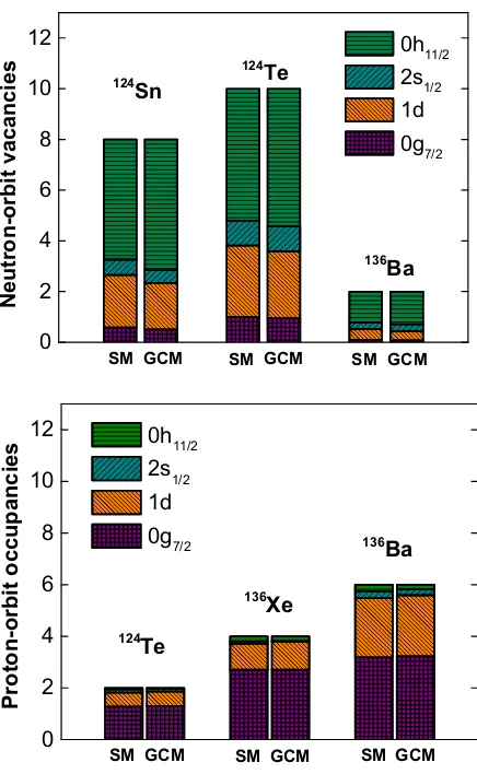
It is known that the 0νββ NMEs are sensitive to the occupancies of valence neutron and proton orbits [33]. To further verify how suitable the Hamiltonian-based GCM is in describing the nuclear structure and 0νββdecay

as-0

FIG. 2: The calculated vacancies of valence neutron orbits for 124_Sn,124_{Te, and}136_{Ba, as well as the calculated occupancies}

of valence proton orbits for124 Te136

Xe, and136 Ba.

pects of the nuclei involved, we also calculate the neutron vacancies for124_Sn, 124_Te, 136_{Xe, and} 136_{Ba, as well as}

the proton occupancies for124_{Te and} 136_{Ba. Our results}

presented in Fig. 2 are compared to the SM calculations reported in Figs. 2-4 of Ref. [7] and Fig. 2 of Ref. [8]. The occupation probabilities of the 1d5/2 and 1d3/2 orbitals

are summed up and presented as 1d, which is similar to the references used for comparison. The occupancies ob-tained with our GCM calculations are close to the values calculated by SM. The calculated occupancies, combined with the g.s. energies and level spectra mentioned above, leads us to consider that Hamiltonian-based GCM is suit-able for the description of the relevant nuclear structure aspects for these initial and final nuclei involved in the 0νββ decay.

C. Analysis of the nuclear matrix elements for

124

Sn,130

Te, and 136

Xe

0

FIG. 3: Calculated 0νββ NMEs, compared to the values given by SM (denoted by “ISM-CMU”) [7, 8], EDF-based GCM employed non-relativistic Gogny D1S force (denoted by “NREDF”) [14] and relativistic PC-PK1 force (denoted by “REDF”) [15].

TABLE II: The NMEs obtained with SVD Hamiltonian by using GCM and SM for 124

Sn, 130

Te, and 136

Xe. CD-Bonn SRC parametrization was used.

M0ν

nuclei for 0νββ-decay experiments [24, 25] presents a pressing need for accurate calculations of the 0νββNMEs to guide the experimental effort.

Figure 3 illustrates the our calculated NMEs, com-pared to the values given by the SM and the EDF-based GCM employing non-relativistic Gogny D1S force and relativistic PC-PK1 force. It can be seen that previ-ous GCM calculations produce NMEs which are about two times larger than the SM ones. In contrast, with our Hamiltonian-based GCM calculations we obtain the NMEs that are about only 40% larger than the SM re-sults, significantly reducing the long-debated discrepancy between previous GCM and SM predictions.

To further understand this 40% overestimation given by our GCM calculations, the values for the 0νββdecay NMEs of124_Sn,130_{Te, and} 136_{Xe are listed in Table II,}

where we show the Gamow-Teller, the Fermi, and the

ten--3

FIG. 4: I-pair decomposition: contributions to the Gamow-Teller matrix elements for the 0νββ decay of 124

Sn, 130 Te, and136

Xe from the configurations when two initial neutrons and two final protons have a certain total spinI, compared to SM [7, 8] calculations. CD-Bonn SRC parametrization was used.

sor contributions. Generally, the Fermi and tensor parts of NMEs present good agreement between our GCM cal-culations and SM calcal-culations, while the Gamow-Teller part of NMEs are noticeably larger in our GCM results, resulting in the 40% overestimation in the total 0νββ NMEs.

0.0 0.2 0.4 0.6 0.8 1.0

I_max=11

I_max=4

I_max=2

M

G

T

G

C

M

-M

G

T

S

M

Sn

130

Te

136

Xe

Imax=0

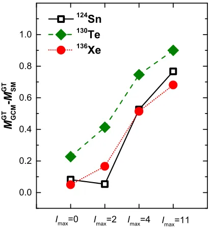
FIG. 5: The differences of Gamow-Teller part of NMEs be-tween our GCM and SM calculations against the pair-spinI

for124 Sn,130

Te, and136 Xe.

at the decomposition of the NMEs over the angular mo-mentumIof the proton (or neutron) pairs (see Eq. (B4) in Ref. [34]), called I-pair decomposition. In this case, the NME can be written as Mα = P_IMα(I), where Mα(I) represent the contributions from each pair-spinI

to the αpart of the NME. To analyse the deviation be-tween the MGT0ν given by GCM and SM, Fig. 4 presents

the I-pair decomposition for the Gamow-Teller part of our calculated 0νββ NMEs, compared to the one calcu-lated by SM [7, 8]. The bars in Figs. 4 can be added directly to get the Gamow-Teller part of NMEs. As we can see, the dramatic cancellation between the I = 0 and I = 2 contributions shown by the SM calculations is reproduced well by our GCM approach. However, SM calculations give more negative contributions withI>4, which further reduce the Gamow-Teller NMEs. On the contrary, our GCM approach can barely produce any con-tributions withI>4.

Figure 5 visualizes the differences in Gamow-Teller NMEs between our GCM and SM calculations against the pair-spinI, which can help us to identify where the differences mainly come from. If we only include the I 6 2 contributions, the Gamow-Teller NMEs obtained by our GCM approach are close to the ones given by SM in all three nuclei involved. However, if the I 64 con-tribution are taken into account, the differences are no-ticeably increased to about 0.5 for124_{Sn and}136_{Xe , and}

about 0.75 for130_{Te. The inclusion of all possible}

pair-spinIcontributions would increase these differences even

NMEs is associated with those large-I-pair contributions, which may correspond to collective or non-collective cor-relations that are excluded from current GCM calcula-tion.

Therefore, the deviation between our current Hamiltonian-based GCM and SM results may be related to the lack of some correlations which become important in 124_Sn, 124_Te, 130_Te, 130_Xe, 136_{Xe, and} 136_{Ba. Since these nuclei are all near spherical or weakly}

deformed, one can expect the non-collective correlations, for example, quasiparticle excitations, may overcome the collective correlations. Currently, the reference states that the GCM method employs are HFB states imposed by the time-reversal symmetry, which exclude any multi-quasiparticle configurations. It would be of great interest if we could treat the quasi-particle excitation as an additional generator coordinate in the future. It could improve the description of 0νββ decay NME for these nuclei.

IV. SUMMARY

In this paper, we present a GCM calculation based on effective shell model Hamiltonians for the 0νββ de-cay NMEs of124_Sn, 130_{Te, and}136_{Xe in thejj55 model}

space that compromises the 0g7/2, 1d5/2, 1d3/2, 2s1/2,

and 0h11/2orbits. We use the SVD effective Hamiltonian

that is fine-tuned with experimental data. To ensure the reliability of the results, we perform the Hamiltonian-based GCM calculations of the ground-state energies, low-lying level spectra, and occupancies of valence neu-tron and proton orbits. These are compared to the SM results obtained by exactly diagonalizing the same effec-tive Hamiltonian. Our results are in reasonable agree-ment with the values obtained with the shell model. We also provide a detailed analysis of 0νββdecay NMEs for

124_Sn, 130_{Te, and}136_{Xe. Our Hamiltonian-based GCM}

produces 0νββ decay NMEs that are about 40% larger than the ones obtained by SM, significantly reducing the large deviation between previous GCM and SM predic-tions. By checking the decomposition of the NMEs over the angular momentumI of the proton or neutron pairs, we find that the remaining 40% overestimation of 0νββ decay NMEs may be associated with the exclusion of some non-collective correlations.

Acknowledgments

Support from the U.S. Department of Energy Topical Collaboration Grant No. de-sc0015376 is acknowledged.

[1] F. T. Avignone III, S. R. Elliott, and J. Engel, Rev. Mod. Phys.80, 481 (2008).

[3] P. Vogel, J. Phys. G39, 124002 (2012).

[4] Y. Iwata, N. Shimizu, T. Otsuka, Y. Utsuno, J. Men´edez, M. Honma, and T. Abe, Phys. Rev. Lett.116, 112502 (2016).

[5] R. A. Sen’kov and M. Horoi, Phys. Rev. C93, 044334 (2016).

[6] J. Men´edez, A. Poves, E. Caurier, and F. Nowacki, Nucl. Phys. A818, 139 (2009).

[7] A. Neacsu and M. Horoi, Phys. Rev. C91, 024309 (2015). [8] M. Horoi and A. Neacsu, Phys. Rev. C93, 024308 (2016). [9] J. Barea, J. Kotila, and F. Iachello, Phys. Rev. C 91,

034304 (2015).

[10] M. T. Mustonen and J. Engel, Phys. Rev. C87, 064302 (2013).

[11] F. ˇSimkovic, V. Rodin, A. Faessler, and P. Vogel, Phys. Rev. C87, 045501 (2013).

[12] J. Hyv¨arinen and J. Suhonen, Phys. Rev. C91, 024613 (2015).

[13] T. R. Rodr´ıguez and G. Mart´ınez-Pinedo, Phys. Rev. Lett.105, 252503 (2010).

[14] N. L. Vaquero, T. R. Rodr´ıguez, and J. L. Egido, Phys. Rev. Lett.111, 142501 (2013).

[15] J. M. Yao, L. S. Song, K. Hagino, P. Ring, and J. Meng, Phys. Rev. C91, 024316 (2015).

[16] N. Hinohara and J. Engel, Phys. Rev. C90, 031301(R) (2014).

[17] J. Men´edez, T. R. Rodr´ıguez, G. Mart´ınez-Pinedo, and A. Poves, Phys. Rev. C90, 024311 (2014).

[18] M. Bender, T. Duguet, and D. Lacroix, Phys. Rev. C79, 044319 (2009).

[19] N. Tsunoda, K. Takayanagi, M. Hjorth-Jensen, and T. Otsuka, Phys. Rev. C89, 024313 (2014).

[20] P. Vogel and M. R. Zirnbauer, Phys. Rev. Lett.57, 3148 (1986).

[21] J. Engel, P. Vogel, and M. R. Zirnbauer, Phys. Rev. C

37, 731 (1988).

[22] J. Men´edez, N. Hinohara, J. Engel, G. Mart´ınez-Pinedo, and T. R. Rodr´ıguez, Phys. Rev. C93, 014305 (2016). [23] C. F. Jiao, J. Engel, J. D. Holt, submitted to Phys. Rev.

C.; arXiv:1707.03940 (2017).

[24] V. Nanal, inInternational Nuclear Physics Conference, INPC 2013, Vol. 2, Firenze, Italy, June 2?7, 2013, EPJ Web of Conferences, Vol. 66 (2014), p. 08005.

[25] D. R. Artusaet al. (CUORE), Eur. Phys. J. C74, 3096 (2014).

[26] F. ˇSimkovic, A. Faessler, H. M¨uther, V. Rodin, and M. Stauf, Phys. Rev. C79, 055501 (2009).

[27] F. ˇSimkovic, A. Faessler, V. Rodin, P. Vogel, and J. En-gel, Phys. Rev. C77, 045503 (2008).

[28] A. L. Goodman, in Advances in N uclear P hysics, edited by J. V. Negele and E. Vogt, (Plenum Press, New York, 1979), Vol. 11, p. 263.

[29] P. Ring and P. Schuck, T he N uclear M any-Body P roblem(Springer-Verlag, Berlin, 1980).

[30] T. R. Rodr´ıguez and J. L. Egido, Phys. Rev. C81, 064323 (2010).

[31] J. M. Yao, J. Meng, P. Ring, and D. Vretenar, Phys. Rev. C81, 044311 (2010).

[32] Chong Qi and Z. X. Xu, Phys. Rev. C86, 044323 (2012). [33] F. ˇSimkovic, A. Faessler, and P. Vogel, Phys. Rev.C79,

015502 (2009).