Full Terms & Conditions of access and use can be found at
http://www.tandfonline.com/action/journalInformation?journalCode=ubes20
Download by: [Universitas Maritim Raja Ali Haji] Date: 11 January 2016, At: 22:12
Journal of Business & Economic Statistics
ISSN: 0735-0015 (Print) 1537-2707 (Online) Journal homepage: http://www.tandfonline.com/loi/ubes20
Unconditional Quantile Treatment Effects Under
Endogeneity
Markus Frölich & Blaise Melly
To cite this article: Markus Frölich & Blaise Melly (2013) Unconditional Quantile Treatment Effects Under Endogeneity, Journal of Business & Economic Statistics, 31:3, 346-357, DOI: 10.1080/07350015.2013.803869
To link to this article: http://dx.doi.org/10.1080/07350015.2013.803869
View supplementary material
Accepted author version posted online: 16 May 2013.
Submit your article to this journal
Article views: 579
View related articles
Unconditional Quantile Treatment Effects
Under Endogeneity
Markus F
ROLICH¨
Department of Economics, Universit ¨at Mannheim, D-68131 Mannheim and IZA, 53113 Bonn, Germany ([email protected])
Blaise M
ELLYDepartment of Economics, Universit ¨at Bern, Schanzeneckstrasse 1, 3001 Bern, Switzerland ([email protected])
This article develops estimators for unconditional quantile treatment effects when the treatment selection is endogenous. We use an instrumental variable (IV) to solve for the endogeneity of the binary treatment variable. Identification is based on a monotonicity assumption in the treatment choice equation and is achieved without any functional form restriction. We propose a weighting estimator that is extremely
simple to implement. This estimator is rootnconsistent, asymptotically normally distributed, and its
variance attains the semiparametric efficiency bound. We also show that including covariates in the estimation is not only necessary for consistency when the IV is itself confounded but also for efficiency when the instrument is valid unconditionally. An application of the suggested methods to the effects of fertility on the family income distribution illustrates their usefulness. Supplementary materials for this article are available online.
KEY WORDS: Instrumental variables; Local average treatment effect (LATE); Nonparametric regression.
1. INTRODUCTION
In many research areas, it is important to assess the dis-tributional effects of policy variables. From a policy perspec-tive, an intervention that helps to raise the lower tail of an income distribution is often more appreciated than an interven-tion that shifts the median, even if the average treatment effects of both interventions are identical. Quantile treatment effects (QTEs) are able to characterize the heterogeneous impacts of variables on different points of the outcome distribution, which makes them appealing in many economics applications. When the treatment of interest is endogenous, instrumental variable (IV) methods provide a powerful tool to identify causal ef-fects. In this article, we consider a nonparametric IV model for QTEs.
Our approach to IV is based on the framework developed by Imbens and Angrist (1994) and Abadie (2003) for a binary treatment and a binary instrument. In this setup, our population of interest is the population of all compliers, which is the largest population for which the effects are point identified. We suggest IV estimators forunconditionalQTEs for compliers. We define the unconditional QTE as the difference between the quantiles of the marginal potential distributions of the treatment and control responses. This is a standard estimand in the evaluation litera-ture, suggested first by Doksum (1974) and Lehmann (1974). Unconditional QTEs can be easily explained using randomized controlled trials as a thought experiment: they represent the distributions of the outcome that would have materialized if hy-pothetically the entire population had been assigned either to treatment or to control (in the absence of general equilibrium effects). In contrast to our approach, a large part of the literature has consideredconditionalQTEs, that is, the effects conditional on the covariatesX.
While conditional and unconditional averagetreatment ef-fects have similar meanings because of the linearity of the ex-pectation operator, this is not the case forquantiles. In a simple example relating wages to years of education, the unconditional 0.9 quantile refers to the high wage workers (most of whom will have many years of schooling), whereas the 0.9 quantile conditional on education refers to the high wage workerswithin
each education class, who however may not necessarily be high earners overall. Presuming a strong positive correlation between education and wages, it may well be that the 0.9 quantile among high school dropouts is lower than, say, the median of all Ph.D. graduates. The interpretation of the 0.9 quantile is thus different for conditional and unconditional quantiles.
The unconditional QTEs are the right estimands to consider when the ultimate object of interest is the unconditional distri-bution. While the welfare of the (unconditionally) poor attracts a lot of attention in the political debate, the welfare of highly educated people with relatively low wages catches much less interest. In this case, the lower end of the unconditional QTE functions will be most interesting to the public debate. In public health, the analysis of the determinants of low birth weight gives another example where we are interested in the unconditional distribution. We are especially concerned with the lower tail of the birth weight distribution, and in particular with cases that fall below the 2500 g threshold.
This is not to say that conditional QTEs are unimportant. Con-ditional QTEs are also of interest in many applications. They allow analyzing the heterogeneity of the effects with respect to
© 2013American Statistical Association Journal of Business & Economic Statistics July 2013, Vol. 31, No. 3 DOI:10.1080/07350015.2013.803869
346
the observables. For example, they can be used to decompose the total variance in a within and a between component. On the other hand, unconditional QTEs aggregate the conditional ef-fects for the entire population. The unconditional quantile func-tions are one-dimensional funcfunc-tions, whereas the conditional quantile functions are multi-dimensional (unless one imposes functional form restrictions). They are more easily conveyed to the policy makers and the public but at the cost of not showing any information about the relationship between the covariates and the outcome.
Because the unconditional effects are averages of conditional effects, they can be estimated more precisely. Unconditional QTEs can be estimated at the√n rate without any paramet-ric assumption, which is obviously impossible for conditional QTEs (unless allXare discrete). Finally, the definition of the un-conditional effects does not depend on the variables included in
X. One can therefore consider different sets of control variables
Xand still estimate the same object, which is useful for exam-ining robustness of the results to the set of control variables.
An alternative motivation for considering quantile effects is the well-known robustness to outliers of quantile estimators (in particular median estimators). Hence, even if one is not primarily interested in the distributional impacts, one may still like to use the methods proposed to estimate median instead of mean treatment effects. This argument is particularly useful for noisy outcomes such as wages or earnings. The quantiles are well defined even if the outcome variable does not have finite moments due to fat tails. This robustness was the first motivation for considering median instead of mean regression in Koenker and Bassett (1978), see also the discussion in Koenker (2005).
Our approach to IV is based on the framework developed by Imbens and Angrist (1994) and Abadie (2003). We assume that the instrument is independent of the outcome variable only con-ditionallyonX. For example, Rosenzweig and Wolpin (1980) and Angrist and Evans (1998) used twin birth as an instrument for family size. Yet, the probability of twin birth depends on race and increases with age. Without controlling for covariates, the IV estimator would be inconsistent. We focus on a binary instrument, yet mention that the setup also permits nonbinary scalar instruments.
Even if there is no need to include covariates for consistency reasons, incorporating covariates is helpful to reduce variance. We show that covariates increase the precision of the estimates. Naturally, our results also cover the case where the instrument is valid unconditionally, for example, a randomized controlled trial. Here, covariates are not needed for consistency, but can still be used to improve precision. These results can be combined by including some covariates to obtain consistency and additionally others for efficiency reasons.
Abadie (2003) gave a general identification result for compli-ers in Theorem 3.1. His instrument probability weighted repre-sentation identifies unconditional QTEs for a specific loss func-tion. We give alternative representations of the estimand, which lead naturally to several types of fully nonparametric estimators: regression (or matching) on the covariates, regression on the in-strument probability, or a weighted version of the traditional quantile regression algorithm proposed by Koenker and Bassett (1978). We show that the proposed nonparametric weighting es-timator is√nconsistent, asymptotically normal, and efficient. In addition to deriving the theoretical properties of the estimator,
we also provide codes written in Stata, which should consider-ably simplify the use of the results derived in this article.
Finally, we present an empirical illustration of the theoreti-cal results. We use U.S. Census data from 2000 to estimate the effects of fertility on family income using twin birth as an instru-ment for the second child. We find that the presence of a second child decreases the family income below the 6th decile but in-creases it above the 6th decile. The IV results are significantly different from the results assuming exogeneity of fertility. The working paper version of this article presents also the lessons drawn from Monte Carlo simulations and two other empirical applications.
We are obviously not the first to consider the estimation of QTEs. This topic has been an active research area during the last three decades. Koenker and Bassett (1978) proposed and derived the statistical properties of a parametric (linear) es-timator for conditional quantile models. Due to its ability to capture heterogeneous effects, its theoretical properties have been studied extensively and it has been used in many empiri-cal studies; see, for example, Powell (1986), Guntenbrunner and Jureˇckov´a (1992), Buchinsky (1994), Koenker and Xiao (2002), and Angrist, Chernozhukov, and Fern´andez-Val (2006). Chaud-huri (1991) analyzed nonparametric estimation of conditional QTEs. All these estimators assume that the treatment selec-tion is exogenous, often labeled as “selecselec-tion-on-observables,” “conditional independence,” or “unconfoundedness.” However, in observational studies, the variables of interest are often en-dogenous. Therefore, AAI (Abadie, Angrist, and Imbens2002) and Chernozhukov and Hansen (2005, 2006, 2008) had pro-posed linear IV quantile regression estimators. Chernozhukov, Imbens, and Newey (2007) and Horowitz and Lee (2007) had considered nonparametric IV estimation of conditional quantile functions. In a series of papers, Chesher (2003,2005,2010) also examined nonparametric identification of conditional effects.
The literature discussed so far dealt with the estimation of conditional QTEs. EstimatingunconditionalQTEs under a selection-on-observables assumption has been the focus of var-ious papers: Firpo (2007) suggested a propensity score weight-ing estimator, Fr¨olich (2007b) a propensity score matching es-timator, and Chernozhukov, Fern´andez-Val, and Melly (2007) derived the properties of a class of regression estimators. We contribute to this literature by allowing the binary treatment to beendogenous. Firpo, Fortin, and Lemieux (2007) nonparamet-rically identified the unconditional effects of marginal changes in the distribution of the explanatory variables, when all vari-ables are exogenous. Unconditional effects with endogeneity for acontinuoustreatment variable have been examined in Rothe (2010) or Imbens and Newey (2009).
Section2presents the model, Section3discusses identifica-tion and suggests nonparametric estimators. Asymptotic prop-erties are examined in Section 4, and Section 5 provides the empirical application, followed by a brief conclusion in Section 6. An online appendix with proofs and additional material is available from the authors’ webpages.
2. NOTATION AND FRAMEWORK
We are interested in the distributional effect of a binary treat-ment variableDon a continuous outcome variable Y. Let Y1 i andY0
i be the potential outcomes of individuali. We focus our
attention on QTEs as they represent an intuitive way to summa-rize the distributional impact of a treatment:
τ=QτY1−Q
τ Y0,
where Qτ
Yd is theτ quantile ofY
d. We identify and estimate
separately the entire quantile processes forτ ∈(0,1). Therefore, our results are not limited to QTEs but extend directly to any functional of the marginal distributions as, for example, the effects on inequality measures such as the Gini coefficient or the interquartile spread as special cases.
We permit Dto be endogenous, and identification will be achieved via an IVZ. Since we allow the treatment effect to be arbitrarily heterogeneous, we are only able to identify effects for the population that responds to a change in the value of the instrument. We therefore focus on the QTEs for thecompliers:
τc =QτY1|c−QτY0|c, (1)
where Qτ
Yd|c is the τ quantile of Y
d in the subpopulation of
compliers, as defined in the following. Although we condition on being a complier, we will refer toτ
c as anunconditional treatment effect because we do not condition here on the other covariatesXintroduced below.
We focus on abinaryinstrumentZhere and mention that the working paper version of this article describes how nonbinary instruments can be accommodated. LetDizbe the potential treat-ment state ifZihad been externally set toz. WithDandZbeing both binary, we can partition the population into four groups defined byDi0andD1i. We define these four types asTi =a if (defiers). Hence, thecompliersare the individuals who respond in the intended way to a change inZ. We assume:
Assumption 1.
(i) Existence of compliers: Pr(T =c)>0 (ii) Monotonicity: Pr(T =d)=0 (iii) Independent instrument: (Y0,T)
⊥⊥Z|X and (Y1,T) ⊥⊥Z|X
(iv) Common support: Supp(X|Z=1)=Supp(X|Z=0)
We will use the shortcut notationPc=Pr(T =c) andπ(x)=
Pr(Z=1|X=x). We will often refer toπ(x) as the “instrument probability.” Assumption 1 is basically the same as in Abadie (2003) and has also been used in Imbens and Angrist (1994), Abadie, Angrist, and Imbens (2002), Abadie (2002), Fr¨olich (2007a), and Kitagawa (2009). The main difference is that As-sumption 1(i) is needed only unconditionally.
Assumption 1(i) requires that at least some individuals re-act to changes in the value of the instrument. The strength of the instrument can be measured byPc, which is the probability mass of the compliers. Assumption 1(ii) is often referred to as monotonicity. It requires that Dizweakly increases with zfor all individuals (or decreases for all individuals). We could alter-natively assume homogeneity between compliers and defiers, that is, FYd|X=x,T=c=FYd|X=x,T=d for d ∈ {0,1} and almost every x. This alternative assumption would lead to the same estimators. Assumption 1(iii) is the main IV assumption. It im-plicitly requires an exclusion restriction and an unconfounded instrument restriction. In other words,Zi should not affect the
potential outcomes of individualidirectly, and those individuals for whomZ=zis observed should not differ in their relevant unobserved characteristics from individuals withZ=z. Often such an assumption is only plausibleconditionalon some co-variatesX. Note further that we donotneedXto be exogenous, that is,Xcan be correlated with the unobservables. For instance,
Xmay contain lagged-dependent variables that may be corre-lated with unobserved ability; see, for example, Fr¨olich (2008). Assumption 1(iv) requires the support ofXto be identical in the Z=0 and theZ=1 subpopulations. If the support condition is not met initially, we need to define the parameters relative to the common support.
Finally, for well-behaved asymptotic properties of the QTE estimators defined later, we will also need to assume that the quantiles are unique and well defined:
Assumption 2. The random variablesY1andY0are contin-uously distributed with positive density in a neighborhood of QτY1|candQ
τ
Y0|cin the subpopulation of compliers.
3. IDENTIFICATION AND ESTIMATION
3.1 Identification
Lemma 1. Under Assumption 1, the distribution ofY1for the compliers is nonparametrically identified as
FY1|c(u)=
The distribution ofY0for the compliers is identified analogously ifDis replaced with 1−Din the numerator and denominator of Equations (2)–(4).
This identifies the QTEs as the difference between the quantiles:
cτ =FY−11|c(τ)−F−
1 Y0|c(τ).
Alternatively,τ
c is directly identified by the following opti-mization problem
The proof of Lemma 1 follows from Theorem 3.1 of Abadie (2003) by noting that our weightsWare the sum of the weights κ(0)andκ(1)suggested in this theorem. Since our Assumption 1 is slightly weaker than his assumptions, some straightforward minor adjustments to the proof are needed.
Note that by Assumption 1, we have thatE[W]=2Pc>0. If the instrument had the reverse effect in that there are defiers but no compliers, we would have to redefine the instrument or alternatively multiply the weights with−1 to haveE[W]>0. Otherwise the optimization (6) would have the wrong sign.
3.1.1 Intuition for the Identification Result. In the follow-ing we convey some intuition for the results in Lemma 1. If Assumption 1 was valid without conditioning onX, the distri-bution function ofY1for the complier subpopulation would be identified by
E[1 (Y ≤u)D|Z=1]−E[1 (Y ≤u)D|Z=0] E[D|Z=1]−E[D|Z=0] .
This unconditional distribution function could then be inverted to obtain the unconditional quantile function. Since a similar re-sult applies to the distribution ofY0, identification of the QTEs would directly follow from this simple result. Now consider the case where Assumption 1 is valid conditional on X. Ob-viously, the distribution function ofY1 for the compliers with characteristicsX=xis analogously identified:
FY1|X=x,T=c(u)=
E[1(Y ≤u)D|X=x, Z=1]−E[1(Y ≤u)D|X=x, Z=0]
E[D|X=x, Z=1]−E[D|X=x, Z=0] (7)
We can, thus, identify the treatment effect for the compliers with characteristicsX=x.
However, we are interested in theunconditionaleffect, that is, the distribution for the subpopulation ofallcompliers (ir-respective of their value of x), which is the largest popula-tion for which the effect is identified. The simple integra-tion
FY1|X,T=c(u)dFX of the conditional distribution using the observable distribution ofXdoes not provide the solution to this problem. Moreover, an estimator based on (7) which uses nonparametric plug-in estimators for all conditional ex-pectations appearing in the formula could have rather poor finite sample properties since the estimate of the denomina-tor of (7) can be close to zero for some values of x. If we want to obtain the unconditional distribution for the compli-ers, we need to weight the conditional distribution by the den-sitydFX|T=cofXamong the compliers. We do not know who
The matching and weighting representations (3) and (4) can be obtained via iterated expectation arguments. To show (6), we note thatFY1|T=c(QτY1|c)=τ such that the quantileQ
could estimate the treatment effect directly by the weighted quantile regression given in (6).
3.2 Estimators
In Section4, we define precisely a weighting estimator and an-alyze its asymptotic properties. In this section, we mention that Lemma 1 suggests several nonparametric estimators. To imple-ment the expression (2), we could estimateE[D|X=x, Z=1] andE[1 (Y ≤u)D|X=x, Z=1] by local logistic regressions or other nonparametric first step estimators. Such estimators can be denoted as regression (or matching) estimators because they correspond to a function of several nonparametric regressions on X. Alternatively, we could use Equation (3) that exploits that controlling for the one-dimensional instrument probability π(X) is sufficient. If the instrument probability is known or if a parametric functional form can be assumed for it, then match-ing on the instrument probabilityπ(X) has the advantage that it does not require high-dimensional nonparametric regressions. Instead of regressing onπ(X), the estimated instrument proba-bilities can alternatively be used to reweight the observations in the sample analog of (4).
The estimators discussed so far will lead to asymptotically monotone estimates ofFY0|c(u) andFY1|c(u). In finite samples,
however, the estimates ofFY0|c(u) andFY1|c(u) are often
non-monotone. This poses problems for the inversion of the cdfs to obtain the quantile functions. We suggest using the method of Chernozhukov, Fernandez-Val, and Galichon (2010) to mono-tonize the estimated distribution functions ˆFY0|c(u) and ˆFY1|c(u)
via rearrangement. These rearrangements do not change the asymptotic properties of the estimators. The rearrangement pro-cedure consists of a sequence of closed-form steps and is fast.
The estimators sketched so far estimate the distribution func-tions (and thus are also applicable to noncontinuous outcome variables). Alternatively we can estimate the quantiles directly. A weighted quantile regression estimator is given by the sam-ple analog of (6). Note that the sample objective function is typically nonconvex sinceWis negative forZ=D. This com-plicates the optimization problem because local optima could exist. AAI noticed a similar problem in their approach but our problem is less serious here because we need to estimate only a
scalarin theD=1 population and another scalar in theD=0 population. In other words, we can write (6) equivalently as
which are two separateone-dimensionalestimation problems in the D=1 and D=0 populations such that we can easily use grid-search methods supported by visual inspection of the objective function for local minima.
Although the negativity of some of the weightsW is not a serious problem, we could follow the approach of AAI to use projected weights. Applying an iterated expectations argument
to (6), we obtain
QτY0|c,
τ c
=arg min a,b
E[ρτ(Y −a−bD)·W+],
where
W+=E[W|Y, D]=E
Z
−π(X)
π(X) (1−π(X))|Y, D
(2D−1).
(9)
These new weights W+ are always nonnegative as shown in the Appendix. Hence, they can be used to develop an estimator with a linear programming representation. The sample objective function to (6) withW+instead ofW is globally convex since it is the sum of convex functions, and the global optimum can be obtained in a finite number of iterations. However, we would need to estimate the positive weights (9) first. Note that AAI suggested a similar projection approach, but their weights are conditional onY, D, andX. Hence, nonparametric estimation of their weights is more difficult and computationally demanding, whereas estimation of (9) requires onlyunivariate nonparamet-ric regression separately for theD=0 andD=1 populations.
3.3 Relationship to the Existing Literature
3.3.1 Relationship to Estimation of QTEs Under Exogeneity. Consider first the special case of our model when the treatmentDis exogenous conditional onX. In this case, we can use Das its own instrument and setZ=Dsuch that our representation in (2) simplifies to
FY1(u)=
E[1 (Y ≤u)|X, D=1]dFX.
(Note that in this situation everyone is a complier.) When the conditional distribution is estimated by parametric methods, we obtain the estimators studied by Chernozhukov, Fern´andez-Val, and Melly (2007). When the conditional distribution is estimated by local regression or by nearest neighbor regression, we obtain the estimator proposed, for example, in Fr¨olich (2007b).
Furthermore, in this exogenous case, our weights simplify to
W = D π(x)+
1−D 1−π(x)
and our expression (6) corresponds to the estimator of Firpo (2007), who proposed using these weights to estimate the QTEs of an exogenous treatment.
3.3.2 Relationship to Abadie, Angrist, and Imbens (2002). For endogenous treatment choice, AAI had proposed an estima-tor for conditional QTEs. Our weighting representation in (6) bears some resemblance with AAI, who suggested estimating a weighted linear quantile regression
arg min α,β
E
ρτ(Y −αD−β′X)·WAAI
WAAI=1−D(1−Z) 1−π(X)−
(1−D)Z
π(X) . (10)
However, both the model and the estimand are different. They imposed a linear parametric specification, whereas our approach is entirely nonparametric. They identified conditional effects, whereas we are interested in unconditional effects. One can
show that if one uses the weightsWAAIin Lemma (1), that is, to run a weighted quantile regression ofYon a constant andD
with weightsWAAI, one estimates
FY−11|c,D=1(τ)−F−
1 Y0|c,D=0(τ)
and not the QTEs
cτ =FY−11|c(τ)−F−
1 Y0|c(τ).
Hence, generally one cannotuse the weightsWAAIto estimate unconditional QTEs. There is one special case, though, where the weightsWAAIwould identify the unconditional QTEs: when the IV is independent ofXsuch that we can writeπ(X)=π. In this case, the following relationship between the weightsW, defined in (5), andWAAIcan be shown as
WAAI=(Dπ+(1−D) (1−π))W.
This implies that, conditionally onD, the weightW is a mul-tiple ofWAAI. Since multiplying with a positive constant does not change the result of the minimization and since the uncondi-tional quantiles for the compliers can be estimated by univariate weighted quantile regression separately in theD=0 and the D=1 population,WAAIandWwould provide the same results in this special case.
3.3.3 Relationship to Other Nonseparable Models. The potential outcomes framework can also be expressed in the jar-gon of the recent literature on nonparametric identification of nonseparable models. We consider a triangular model as in Im-bens and Newey (2009)
Yi =ϕ(Di,Xi, Ui) (11)
Di =ζ(Zi,Xi, Vi),
where U andV are possibly dependent unobservables and X
are additional covariates, which arepermitted to be correlated withUand/orV. We assume that, after having includedXin the model,Z is excluded from the functionϕ. The corresponding potential outcomes are
Yid =ϕ(d,Xi, Ui)
Diz=ζ(z,Xi, Vi).
In contrast to Chernozhukov and Hansen (2005), Chernozhukov, Imbens, and Newey (2007), and Chesher (2010), we impose tri-angularity, that is, assume thatYdoes not enter inζ. On the other hand, we donot need to assume any kind of monotonicity or rank invariance forϕ. We do impose, however, that the function ζis weakly monotone in its first argument and normalize it to be weakly increasing, that is, assume that an exogenous increase inZican never decrease the value ofDi. This is the monotonic-ity assumption of Imbens and Angrist (1994). This assumption may be more plausible than monotonicity inϕ in some appli-cations, whereas in other applications it may be less appealing. In some applications, monotonicity ofζ is satisfied by design, for example, in trials where only one-sided noncompliance is possible.
Imbens and Newey (2009) developed an alternative identi-fication approach for Model (11) assuming that ζ is mono-tone in its third argument. However, point identification is achieved only when ζ is strictly monotone, which is only
sensible for a continuous treatment variable D, whereas we focus on binaryD.
4. ASYMPTOTIC PROPERTIES
In the previous section several estimators have been sug-gested. In this section, we analyze the asymptotic properties of the weighting estimator, which is the simplest one to implement since it requires only one nonparametric regression. We also show that the estimator is efficient.
From (6), a natural estimator ofτ
For this we need a first step estimator of the weights ˆWi, which depends on a nonparametric estimate ofπ(x). For concreteness, we develop the asymptotic distribution for ˆπ(x) being estimated bylocal linear regression.
Note that the asymptotic distribution does not depend on the specific nonparametric estimator used to estimateπ(x). In the working paper version of this article, we also consider ex-plicitly local logitregression. Alternative nonparametric esti-mators could be used as well, but local linear regression has several appealing properties. It has better boundary properties than Nadaraya–Watson regression and is easier to implement than local higher order polynomial regression, particularly when dim(X) is large. Another alternative is series regression. The use of series methods as, for example, in Hirano, Imbens, and Ridder (2003) or Firpo (2007), however, seems to require very strong smoothness assumptions. For example, Firpo (2007) required more than seven times dim(X) continuous derivatives of the propensity score. To make his treatment exogeneity assumption plausible, usually manyXvariables are needed. Since our esti-mator includes Firpo (2007) as a strict special case forZ=D, our results also complement his article when local linear esti-mation is used instead of series regression.
The local linear regression estimator ofπ(x0) at a locationx0 is defined as the value ofathat solves the weighted least-square regression
whereKj is the product kernel
Kj =Kh(Xj−x0)=
x0. Further,κis a univariate kernel function of orderλ, which is
assumed to be integrating to one. The following kernel constants will be used later:μt =
Assumption 3 gives regularity conditions under which the estimator is asymptotically normal and efficient. We only deal withcontinuouscovariatesX, that is, we assume that the co-variatesXare continuously distributed with a Lebesgue density. This is an assumption made for convenience to ease the exposi-tion. Discrete covariates can easily be included inXand do not change the asymptotic properties. Note that for identification we donotrequire any continuousXvariables.
Assumption 3.
(i) The data{(Yi, Di, Zi,Xi)}are iid fromR×R×R×X withX ⊂RLbeing a compact set.
(ii) c < π(x)<1−coverX for somec >0. (iii) Smoothness:
- π(x) is 2 times continuously differentiable with second derivative H¨older continuous,
- f(x) is λ−1 times continuously differentiable with (λ−1)th derivative H¨older continuous,
(iv) Uniform consistency: The estimator ˆπ(x) satisfies
sup x∈X|
ˆ
π(x)−π(x)|−→p 0.
(v) The univariate kernel functionκis compactly supported, bounded, Lipschitz, and of orderλ. We also assume that
κ(u)du=1.
(vi) The bandwidth satisfiesnhL/lnn
→ ∞andnh2λ→0.
Since the estimated weights ˆW imply a weighting by the inverses of ˆπ(x) and 1−πˆ(x), we need ˆπ(x) to be bounded away from zero and one. This is implied by Assumption 3(ii) and 3(iv). In Assumption 3(iv), we simply assume ˆπ(x) to be uniformly consistent since there are many different sets of as-sumptions under which local linear estimation can be shown to be uniformly consistent. Some assumptions may be more appro-priate in certain settings, other more in others, see, for example, Fan (1993), Masry (1996), or Gozalo and Linton (2000). For example, if we use a conventional second-order kernel (λ=2), the results of Gozalo and Linton (2000) apply to the local linear estimator. Their Theorem 1(ii) withs=r=0 requiresf(x) to be bounded away from zero and further thatf(x) andπ(x) are continuous. They also require the existence ofE[Z2]<
∞and var(Z|X=x)<∞to be a continuous function ofx, which are trivially satisfied sinceZis Bernoulli.
Assumption 3(v) and 3(vi) are needed to reduce the bias term to a sufficiently small order. Together they require thatλ > L/2. Hence, ifXcontains four or more continuous regressors, higher order kernels, that is, λ >2, are required. With three or less continuous regressors, conventional kernels (λ=2) can be used. We propose to use a product kernel, such that higher order kernels are very convenient to implement in practice. In addition, they conveniently permit to smooth over continuous and discrete regressors as suggested by Racine and Li (2004). Although the asymptotic theory is not affected by discrete regressors and the common solution is to conduct separate regressions within each
cell spanned by the discrete regressors, smoothing over discrete regressors can increase precision in finite samples.
We could permit for a more general kernel function with mul-tiple bandwidths as, for example, in Ruppert and Wand (1994) at the expense of a more complex notation. In practice, it ap-pears to be common to rotate the data beforehand such that the covariance matrix is the identity matrix and to use a common bandwidth, instead of estimating a different bandwidth value for eachXvariable.
The following theorem gives the asymptotic distribution of ˆ
τ
c.It also shows that it is efficient in the class of regular semi-parametric estimators.
Theorem 1(Asymptotic distribution). Under Assumptions 1– 3, the estimator (12) is√nconsistent, asymptotically normal, and efficient:
whereV is equal to
The expression for the asymptotic variance is long because each term appears four times: once in each stratum defined by
D andZ. However, each of these terms is conceptually easy. First, note that the effective sample size is proportional to the number of compliers. Second, it is well known that the variance of a quantile is equal to the variance of the distribution function evaluated at this quantile divided by the squared density at this quantile. Third, since we are interested in the unconditional dis-tribution, by the law of total variance the variance will be the sum of the average conditional variance and the variance of the conditional distribution. The first line of the variance expression corresponds to the average conditional variance where the con-ditional variance of FY is FY(1−FY). The second and the third lines of the variance expression correspond to the average variance of the conditional distribution. If the covariates were irrelevant, the conditional distribution at theτth quantile would be uniformly equal toτand these lines would be equal to 0. Note that the last line takes into account the correlations between the conditional distributions at different values ofDandZ.
The asymptotic varianceV contains the terms fYd|c(Qτ
Yd|c),
π(X),Pc,E[D|X, Z], andFY|D,Z,X(QτYd|c). Even if the formula
looks very complicated, straightforward consistent estimators exist for each element, which can be combined to estimateV.
In contrast to, for example, the asymptotic variance of the linear quantile regression estimator, we do not need to estimate condi-tional densities, which are typically difficult to estimate. On the other hand, we need to estimate theunivariatedensities of the potential distributionsfYd|c(Qτ
Yd|c). As suggested by AAI and
Firpo (2007), we can estimate such a density by a reweighted kernel estimator, using the weights already used to estimate the QTEs. AAI gave regularity conditions under which this estimator is consistent. We have already defined ˆπ(X) and ˆQτ
Yd|c.
Pc is consistently estimated by the sample average of DiWˆi . E[D|X, Z] can be estimated using a similar strat-egy and similar regularity conditions to those used to esti-mate π(x). Methods to estimate the conditional distribution FY|D,Z,X are suggested, for instance, in Hall, Wolff, and Yao (1999). We use their local logit estimator. The estimator of the variance obtained by inserting all these estimators in the asymptotic formula is consistent by the continuous mapping theorem.
Under Assumptions 1–3, the proposed estimator is efficient in the sense of attaining the semiparametric efficiency bound. Using the results of Newey (1994), one can also easily show that the efficiency bound doesnot change when the functionπ(x) happens to be known. In the leading example of experimental trials with imperfect compliance, whereZis randomization into treatment andDis actual treatment receipt, the probabilityπ(x) is usually under the control of the institution conducting the experiment and thereby known. Even in this case, it is better to estimate the instrument probability instead of using the known instrument probability.
Including more variables inX, on the other hand, can reduce the variance bound as shown in the following theorem. Hence, additionalXvariables can help to obtain more precise estimates of unconditional QTEs. We can combine these two results in that we might include some control variables to obtain consistency, that is, to make Assumption 1 valid, and others for efficiency reasons. Consider two regressor setsX1andX2withX1⊂X2. We permit that X1 may be the empty set. Suppose that both regressor sets satisfy Assumption 1. We also suppose for the following theorem that
Pr (Z=1|X1,X2)=Pr (Z=1|X1) . (13)
Hence, theadditional regressors inX2, that is, those that are not included inX1, do not affect the instrument. In other words, these additional regressors are not needed for making the IV assumptions valid. However, these additional variables in X2 increase the precision.
Theorem 2(Variance reduction). LetX1 andX2withX1⊂
X2be two regressor sets that both satisfy Assumptions 1 and 2 as well as Equation (13). LetV1be the semiparametric variance
bound when using regressor setX1andV2be the semiparametric variance bound when using regressor setX2, both referring to the same quantileτ of the QTEs. Then
V1≥V2.
As can be expected,V1 and V2 are equal if Y is
indepen-dent fromX2givenX1. Except for these special circumstances, though, the inequality would generally be strict.
5. EFFECTS OF FERTILITY ON HOUSEHOLD
INCOME
The impact of children on their parents’ labor supply and income is of great interest to economists and demographers, but its estimation is difficult because of the endogeneity of fertility. We use twin births as an instrument for family size to control for unobserved heterogeneity, following an idea introduced by Rosenzweig and Wolpin (1980). We use data from the 1% and 5% Census Public Use Micro Samples (PUMS) from 2000. We limit our sample tomarried women who are between 21 and 35 years old. Since we use twin birth as an instrument for fertility, we limit our sample to women who have at least one child. This dataset was used previously by Vere (2011), who gave detailed information about the sample and some descriptive statistics. Angrist and Evans (1998) used similar samples from the 1980 and 1990 censuses.
Our outcome variable of interestYis the sum of the mother’s and father’s yearly labor incomes in 1999. It includes wages, salary, armed forces pay, commissions, tips, piece-rate pay-ments, cash bonuses earned before deductions were made for taxes, bonds, pensions, union dues, etc. Our treatment variable
Dis equal to one if the mother has at least two children and zero otherwise. The instrumentZis equal to one if a twin birth occurred at the first birth and zero otherwise. Since mothers are not asked directly whether they have given birth to twins,Z
must be imputed from data on the year of birth. The resulting measurement error is very small because only about 2.5% of interpregnancy intervals are below 3 months (see, for instance, Zhu and Le2003) and less than 25% of these births will take place in the same calendar year. Accordingly, the mean of our indicator for twin birth is very close to the twinning rate in the national vital statistical report.
The monotonicity assumption is trivially satisfied in this ap-plication because the presence of twins mechanically implies the presence of at least two children in the family. Hence, there are two types of families in our population: those who have more than one child irrespective of the value ofZand those who have more than one child only when a twin birth occurs. We identify the treatment effects for this latter group, which represents 40% of our population as shown in Table 1. Twin births are rela-tively rare as they represent only 1.5% of the births. However, thanks to the size of the census we have 8572 twin births in our sample, which is sufficient to provide relatively precise point estimates.
The occurrence of a twin birth is random but not completely independent of other characteristics. For example, it is well known that the probability of twin births is higher for black par-ents and increases with the age of the mother. For this reason, we follow the literature and defineXas the vector of mother’s age, race, and education. As a robustness check we later also include similar characteristics of the father and the state of residence of the parents. We estimate the instrument probability by local linear regression. We follow the suggestion made by Racine and Li (2004) of also smoothing over the discrete variables to im-prove precision in small samples. A product Gaussian kernel is
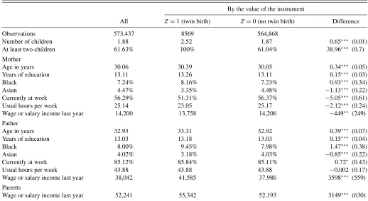
Table 1. Descriptive statistics
By the value of the instrument
All Z=1 (twin birth) Z=0 (no twin birth) Difference
Observations 573,437 8569 564,868
Number of children 1.88 2.52 1.87 0.65∗∗∗ (0.01)
At least two children 61.63% 100% 61.04% 38.96∗∗∗ (0.7)
Mother
Age in years 30.06 30.39 30.05 0.34∗∗∗ (0.05)
Years of education 13.11 13.26 13.11 0.15∗∗∗ (0.03)
Black 7.24% 8.16% 7.23% 0.93∗∗∗ (0.34)
Asian 4.47% 3.35% 4.48% −1.13∗∗∗ (0.22)
Currently at work 56.29% 51.31% 56.37% −5.05∗∗∗ (0.61)
Usual hours per week 25.14 23.05 25.17 −2.12∗∗∗ (0.24)
Wage or salary income last year 14,200 13,758 14,206 −449∗∗ (249)
Father
Age in years 32.93 33.31 32.92 0.39∗∗∗ (0.07)
Years of education 13.03 13.18 13.03 0.15∗∗∗ (0.04)
Black 8.00% 9.45% 7.98% 1.47∗∗∗ (0.38)
Asian 4.02% 3.18% 4.03% −0.85∗∗∗ (0.22)
Currently at work 85.12% 85.84% 85.11% 0.72∗ (0.43)
Usual hours per week 43.88 43.88 43.88 −0.002 (0.17)
Wage or salary income last year 38,042 41,585 37,986 3598∗∗∗ (559)
Parents
Wage or salary income last year 52,241 55,342 52,193 3149∗∗∗ (630)
NOTES: Own calculations using the PUMS sample weights. The sample consists of married mothers between 21 and 35 years of age with at least one child.∗,∗∗,∗∗∗indicate statistical significance at the 10%, 5%, and 1% level, respectively. Standard errors are given in parentheses.
-5
Effects of having more than one child on family income
Figure 1. Unconditional QTEs of having at least two children on family income (defined as gross annual labor income of father plus mother) with pointwise 95% confidence intervals. The sample is taken from the 1% and 5% Census Public Use Micro Samples in 2000 and comprises married women who are between 21 and 35 years old and have at least one child. The instrument is an indicator for twins at the firstbirth.
used. We select the smoothing parameters by cross-validation. Since cross-validation is not consistent for choosing the opti-mal bandwidth, we also examine the sensitivity of the results in Figure A1 of the online supplementary appendix and find that the results are robust to the choice of the bandwidth (especially to smaller bandwidths).
Figure 1reports the estimated QTEs along with 95% point-wise confidence intervals. We estimate the asymptotic standard errors as described in Section 4. The bootstrap standard er-rors reported in Figure A2 (online supplementary materials) are very similar. We find that the QTEs are negative below the 60th percentile and positive above. This heterogeneity is statis-tically significant with most QTEs significantly negative below the median and significantly positive above the 80th percentile. It is also economically significant with estimates ranging from −4000 dollars at the first quartile (this corresponds to−10% of Q0.25Y0|c) up to +10,000 dollars at the 9th decile (+10% of
Q0.90Y0|c).
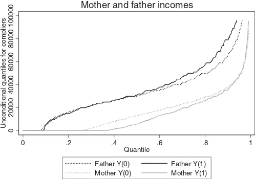
We explain this result by the combination of two effects of fertility. First, the literature has shown that the birth of an additional child leads on average to a reduction in female la-bor supply but does not change male labor supply. Figure 2 shows similar results using our data. The birth of a second child has no noticeable effect on any quantile of the distribution of hours worked by the father. On the other hand, the second child increases the proportion of nonworking mothers by 13%-points. Second, the literature has also shown that fatherhood increases wages; for instance, Lundberg and Rose (2002) found a 6% in-crease in the father’s wage after the birth of the second child. Figure 3shows the potential annual labor income distributions. For men, the income effects are negligible below the median and then increase steadily for higher quantiles. Lundberg (2005) at-tributed this to a compensating differential for less pleasant jobs taken because of increased financial responsibilities and to an increased effort or productivity. The estimated QTEs refer to the subpopulation of compliers, that is, those who had planned
0
Mother and father labor supply
Figure 2. Quantiles of potential outcome distributions of father’s and mother’s annual hours of labor supply.Y(0) is the potential outcome for having one child, whileY(1) is the potential outcome for having at least two children. Labor supply is defined as the product of the number of weeks worked with the usual number of hours worked per week. See also the note belowFigure 1.
to have only one child but ended up with several because of a twin birth. The additional (unplanned) child increases financial needs particularly if one aimed for high quality paid child care, an expensive school and college education, a bigger house with a separate bedroom for each child, etc. Parents who value such investments highly may be willing to take less attractive jobs, for example, longer commuting distances, fewer job amenities, put in more effort to obtain bonus payments, etc. For women, apart from those not working, the effects are negative but turn close to zero for very large quantiles.
Overall, the negative mother hours effect dominates on the lower part of the income distribution whereas the positive fa-ther wage effect dominates on the upper part of the distribution, thereby producing the heterogeneity found in Figure 1. The birth of a child can open a type of poverty trap at the bottom
0
Figure 3. Quantiles of potential outcome distributions of father’s and mother’s annual labor income. Y(0) is the potential outcome for having one child, while Y(1) is the potential outcome for having at least two children. See also the note belowFigure 1.
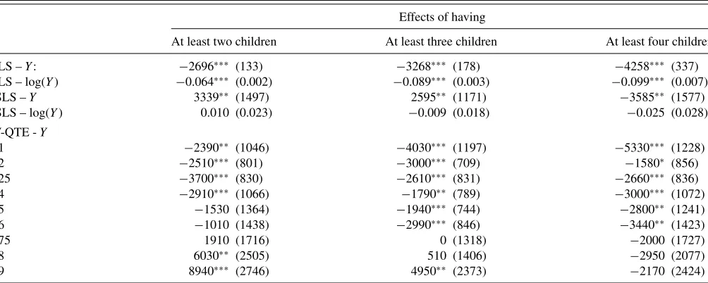
Table 2. Effects of fertility on household income
Effects of having
At least two children At least three children At least four children
OLS –Y: −2696∗∗∗ (133) −3268∗∗∗ (178) −4258∗∗∗ (337) OLS – log(Y) −0.064∗∗∗ (0.002) −0.089∗∗∗ (0.003) −0.099∗∗∗ (0.007)
2SLS –Y 3339∗∗ (1497) 2595∗∗ (1171) −3585∗∗ (1577)
2SLS – log(Y) 0.010 (0.023) −0.009 (0.018) −0.025 (0.028)
IV-QTE -Y
0.1 −2390∗∗ (1046) −4030∗∗∗ (1197) −5330∗∗∗ (1228)
0.2 −2510∗∗∗ (801) −3000∗∗∗ (709) −1580∗ (856)
0.25 −3700∗∗∗ (830) −2610∗∗∗ (831) −2660∗∗∗ (836)
0.4 −2910∗∗∗ (1066) −1790∗∗ (789) −3000∗∗∗ (1072)
0.5 −1530 (1364) −1940∗∗∗ (744) −2800∗∗ (1241)
0.6 −1010 (1438) −2990∗∗∗ (846) −3440∗∗ (1423)
0.75 1910 (1716) 0 (1318) −2000 (1727)
0.8 6030∗∗ (2505) 510 (1406) −2950 (2077)
0.9 8940∗∗∗ (2746) 4950∗∗ (2373) −2170 (2424)
NOTES: The samples are taken from the 1% and 5% Census Public Use Micro Samples (PUMS) in 2000 and comprise married women who are between 21 and 35 years old and have at least one, two, and three children, respectively, for the first, second, and third columns. The instruments are indicators for twins at the first, second, and third birth, respectively. The covariates in the ordinary least square (OLS) and 2SLS regressions are the following: age, age squared, education in years, and high-school, college, black, asian, and other race dummies.Yis the household annual labor income. The IV QTE estimator suggested in this article is invariant to monotone transformations of the dependent variable. The OLS and 2SLS estimators are not invariant; therefore, we present results for the level and the logarithm of the household income as dependent variable. Household income is reported as zero for 4% of the observations used in the first column, for 4.5% of the observations used in the second column, and for 5.9% of the observations used in the last column.
of the distribution, while it simply leads to substitution between leisure and work at the top of the distribution. Standard mean IV estimators, such as two-stage least squares (2SLS), are unable to provide this information. The first column ofTable 2shows the 2SLS estimates of the effect of having more than one child. Since mean IV estimators are not invariant to transformations of the dependent variable, we show the effects onYand log(Y). While the results are significantly positive when the dependent variable isY, the estimates are not significantly different from 0 when using log(Y). Thus, a simple 2SLS analysis hides the heterogeneity found inFigure 1and can be sensitive to a func-tional transformation of the outcome variable.
Figure 4compares the estimates obtained with various alter-native estimators. The solid line labeled “IV with covariates” is the same as that shown inFigure 1. The gray line labeled “IV without covariates” provides the IV estimates when we do not include any covariatesX. Omitting control variables leads to an overestimation of the effects. This is mostly due to the simultaneous positive correlations between age and twinning rate and age and wage. The last two lines show that controlling for endogeneity via IVs is important. The estimated effects are uniformly negative when we assume thatDis exogenous or con-ditionally exogenous (i.e., assuming selection on observables).
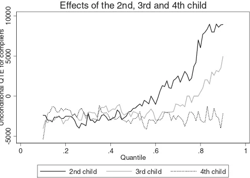
We can use the same strategy to estimate the effects of further children by exploiting twin births in larger families. In addition to the effects of a second child already given inFigure 1,Figure 5 shows the effects of a third and a fourth child, when using twins at the second and third birth, respectively, as an instrument. The overall pattern of the QTEs looks similar, but the positive ef-fects at the higher quantiles dissipate quickly for larger families: while the QTEs are positive for the second child from the 60th percentile onward, for the third child they are positive only from the 80th percentile onward, and for the fourth child there is no
evidence for a positive effect at all. These results are in accor-dance with Lundberg and Rose (2002) who found no positive wage effects after the first two children. While the negative fe-male hours effect persists, the positive wage effect disappears. These results must be interpreted with caution because they re-fer to difre-ferent populations of compliers. The effects of a second child are identified for those families who wanted to have only a
-1
0000
0
100
00
200
00
Unc
ondi
tional Q
T
E
0 .2 .4 .6 .8 1
Quantile
IV with covariates IV without covariates Observed differences Selection on observables
Comparison of estimates
Figure 4. Comparison of four estimators of the unconditional QTEs of having at least two children on family annual labor income. The IV estimator(solid black line) is defined in Section4. The estimates are identical toFigure 1. The covariates included are age, education, and race of the mother. The IV without covariatesestimator is the same estimator without any covariates. TheObserved differencesare the differences between the raw quantiles for families with one child and families with more than one child. TheSelection-on-observables estimator is the estimator suggested by Firpo (2007) and has been implemented with the same covariates.
-5
000
0
50
00
10
000
Unc
o
ndi
tional Q
T
E
f
o
r c
o
m
p
lier
s
0 .2 .4 .6 .8 1
Quantile
2nd child 3rd child 4th child
Effects of the 2nd, 3rd and 4th child
Figure 5. Effects of having at least two, at least three, and at least four children, respectively, on family annual labor income. The solid black line (2nd child) replicates the results ofFigure 1. The samples have been restricted to mothers with at least one, two, and three children, respectively. The instruments are indicators for twins at the first, second, and third birth, respectively. See also the note belowFigure 1.
single child, but ended up with more because of twin birth. The effects of further children refer to families who wanted to have several children from the beginning.
In Figures A3 and A4 (online supplementary materials), we provide two robustness checks with respect to a possible threat to the exogeneity of the twin birth instrument. It had been ob-served that the twinning rate increased during the last 30 years. As discussed by Vere (2011), this increase is first explained by the shift in the maternal age distribution as more women delay childbearing into their late 30s and 40s. It is also not excluded that diet (e.g., bovine growth hormone) affects the probability of having twins. Another possible factor, though, is the increase in the use of assisted reproductive technology (ART), which is associated with a higher twinning probability. Since the use of ART is unobserved in our dataset, this may jeopardize the validity of the instrument if the subset of families using ART differs in their labor earnings from the general population. To deal with this possible threat, we had restricted our population to women 35 years or younger. Their average age at first birth is 24 years. While the use of ART might be an important fac-tor in the older population, it is rather infrequent among young women: Reynolds et al. (2003) wrote “The contribution of ART to twin and triplet/births increased dramatically with maternal age, reflecting that few women early in their reproductive life turn to these techniques to achieve pregnancy.” Using their prob-abilities in Table 4, ART explains only less than 5% of the twin births in our population. Even if this number may understate the true problem due to other fertility-enhancing drugs, it is unlikely to lead to a large bias in our subpopulation studied.
To alleviate remaining concerns, we analyzed this further. First, we checked the robustness of the results to the inclusion of father’s characteristics and state of residence in Figure A3 (online supplementary materials). The results are almost un-changed, showing that father’s characteristics do not affect the twinning probability, which would be the case if ART was an important determinant. In addition, we notice from the medical
literature that fertility-enhancing technologies increase almost only the probability of having dizygotic twins. Hence, as a fur-ther robustness check, we use only same-sex twins as an instru-ment. The results in Figure A4 (online supplementary materials) remain rather similar.
6. CONCLUSIONS
In this article, we have examined a nonparametric endoge-nous treatment effect model. The presence of a binary IV to-gether with a monotonicity assumption in the selection equation identifies the treatment effect for the compliers. We make three contributions to the literature. First, we suggest looking at a different estimand than the estimands considered so far. Uncon-ditional QTEs (for compliers) are relevant in many applications where the final object of interest is defined independently of the value of the covariates. For instance, most policy makers care about families below the poverty line or about babies below the low birth weight threshold. These two populations are defined independently from the value of the covariates. In addition, the unconditional QTEs are easy to convey and can be estimated precisely even without functional form assumptions.
In our framework, the general result of Abadie (2003) implies identification of the unconditional QTEs. Our second contribu-tion is to suggest a nonparametric estimator and to show that it is rootnconsistent, asymptotically normally distributed, and efficient. This estimator is easy to implement and requires only estimating a single nonparametric regression. We also show that including relevant covariates that are not needed for identifica-tion decreases the asymptotic variance of the estimates. Such a result cannot be derived for conditional QTEs because, in that case, the estimand changes when we include covariates, even when they are not needed for identification.
Finally, this article contributes to the empirical literature on the effects of fertility on households’ labor supply. We apply the suggested procedures to data from the 2000 U.S. Census using twin births as instrument. We find strong heterogeneity in the causal effect of childbearing on the household income. While the effects of having at least two children has a negative effect below the 6th decile, it has a positive effect above this quantile.
SUPPLEMENTARY MATERIALS
Figures A1 to A4 are available in the online supplementary material. The proofs of the theorems are available from the authors.
ACKNOWLEDGMENTS
We thank James Vere for providing us with the data for the application. We have benefited from comments by Alberto Abadie, Joshua Angrist, Guido Imbens, Michael Lechner, the editor Keisuke Hirano, an associate editor, and two anonymous reviewers as well as seminar participants at the University of St. Gallen, the IZA Workshop “Heterogeneity in Micro Econo-metric Models,” Harvard, Uppsala, MIT, Georgetown, Brown, Boston University, Pompeu Fabra, Toulouse I, CEMFI, Bocconi, Lausanne, Tilburg, Mannheim. This research was supported by
the German Research Foundation (DFG), Project B5 of the Re-search Center SFB 884.
[Received September 2010. Revised May 2012.]
REFERENCES
Abadie, A. (2002), “Bootstrap Tests for Distributional Treatment Effects in
Instrumental Variable Models,”Journal of the American Statistical
Associ-ation, 97, 284–292. [348]
——— (2003), “Semiparametric Instrumental Variable Estimation of
Treat-ment Response Models,” Journal of Econometrics, 113, 231–263.
[346,347,348,356]
Abadie, A., Angrist, J., and Imbens, G. (2002), “Instrumental Variables Es-timates of the Effect of Subsidized Training on the Quantiles of Trainee
Earnings,”Econometrica, 70, 91–117. [347,348]
Angrist, J., Chernozhukov, V., and Fern´andez-Val, I. (2006), “Quantile Re-gression Under Misspecification, With an Application to the U.S. Wage
Structure,”Econometrica, 74, 539–563. [347]
Angrist, J., and Evans, W. (1998), “Children and Their Parents Labor Supply:
Evidence From Exogeneous Variation in Family Size,”American Economic
Review, 88, 450–477. [347,353]
Buchinsky, M. (1994), “Changes in the U.S. Wage Structure 1963–1987:
Ap-plication of Quantile Regression,”Econometrica, 62, 405–458. [347]
Chaudhuri, P. (1991), “Global Nonparametric Estimation of Conditional
Quan-tile Functions and Their Derivatives,”Journal of Multivariate Analysis, 39,
246–269. [347]
Chernozhukov, V., Fernandez-Val, I., and Galichon, A. (2010), “Quantile and
Probability Curves Without Crossing,”Econometrica, 78, 1093–1125. [349]
Chernozhukov, V., Fern´andez-Val, I., and Melly, B. (2007), “Inference on
Coun-terfactual Distributions,”Econometrica, forthcoming. [347,350]
Chernozhukov, V., and Hansen, C. (2005), “An IV Model of Quantile Treatment
Effects,”Econometrica, 73, 245–261. [347,350]
——— (2006), “Instrumental Quantile Regression Inference for Structural and
Treatment Effect Models,”Journal of Econometrics, 132, 491–525. [347]
——— (2008), “Instrumental Variable Quantile Regression: A Robust Inference
Approach,”Journal of Econometrics, 142, 379–398. [347]
Chernozhukov, V., Imbens, G., and Newey, W. (2007), “Instrumental Variable
Estimation of Nonseparable Models,”Journal of Econometrics, 139, 4–14.
[347,350]
Chesher, A. (2003), “Identification in Nonseparable Models,”Econometrica,
71, 1405–1441. [347]
——— (2005), “Nonparametric Identification Under Discrete Variation,”
Econometrica, 73, 1525–1550. [347]
——— (2010), “Instrumental Variables Models for Discrete Outcomes,”
Econo-metrica, 78, 575–601. [347,350]
Doksum, K. (1974), “Empirical Probability Plots and Statistical Inference for
Nonlinear Models in the Two-Sample Case,”The Annals of Statistics, 2,
267–277. [346]
Fan, J. (1993), “Local Linear Regression Smoothers and Their Minimax
Effi-ciency,”The Annals of Statistics, 21, 196–216. [351]
Firpo, S. (2007), “Efficient Semiparametric Estimation of Quantile Treatment
Effects,”Econometrica, 75, 259–276. [347,350,351,352,355]
Firpo, S., Fortin, N., and Lemieux, T. (2007), “Unconditional Quantile
Regres-sions,”Econometrica, 77, 953–973. [347]
Fr¨olich, M. (2007a), “Nonparametric IV Estimation of Local Average Treatment
Effects With Covariates,”Journal of Econometrics, 139, 35–75. [348]
——— (2007b), “Propensity Score Matching Without Conditional Indepen-dence Assumption - With an Application to the Gender Wage Gap in the UK,”Econometrics Journal, 10, 359–407. [347,350]
——— (2008), “Parametric and Nonparametric Regression in the Presence of
Endogenous Control Variables,”International Statistical Review, 76, 214–
227. [348]
Gozalo, P., and Linton, O. (2000), “Local Nonlinear Least Squares: Using
Para-metric Information in NonparaPara-metric Regression,”Journal of Econometrics,
99, 63–106. [351]
Guntenbrunner, C., and Jureˇckov´a, J. (1992), “Regression Quantile and
Regres-sion Rank Score Process in the Linear Model and Derived Statistics,”The
Annals of Statistics, 20, 305–330. [347]
Hall, P., Wolff, R. C. L., and Yao, Q. (1999), “Methods for Estimating a
Condi-tional Distribution Function,”Journal of the American Statistical
Associa-tion, 94, 154–163. [352]
Hirano, K., Imbens, G., and Ridder, G. (2003), “Efficient Estimation of Average
Treatment Effects Using the Estimated Propensity Score,”Econometrica,
71, 1161–1189. [351]
Horowitz, J., and Lee, S. (2007), “Nonparametric Instrumental Variables
Es-timation of a Quantile Regression Model,”Econometrica, 75, 1191–1208.
[347]
Imbens, G., and Angrist, J. (1994), “Identification and Estimation of Local
Average Treatment Effects,”Econometrica, 62, 467–475. [346,347,348,350]
Imbens, G., and Newey, W. (2009), “Identification and Estimation of Triangular
Simultaneous Equations Models Without Additivity,” Econometrica, 77,
1481–1512. [347,350]
Kitagawa, T. (2009), “Identification Region of the Potential Outcome Dis-tributions Under Instrument Independence,” Cemmap Working Paper, CWP30/09, Centre for Microdata Methods and Practice, Institute for Fiscal
Studies. [348]
Koenker, R. (2005),Quantile Regression, Cambridge: Cambridge University
Press. [347]
Koenker, R., and Bassett, G. (1978), “Regression Quantiles,”Econometrica, 46,
33–50. [347]
Koenker, R., and Xiao, Z. (2002), “Inference on the Quantile Regression
Pro-cess,”Econometrica, 70, 1583–1612. [347]
Lehmann, E. (1974),Nonparametrics: Statistical Methods Based on Ranks, San
Francisco, CA: Holden-Day. [346]
Lundberg, S. (2005), “Men and Islands: Dealing With the Family in Empirical
Labor Economics,”Labour Economics, 12, 591–612. [354]
Lundberg, S., and Rose, E. (2002), “The Effects of Sons and Daughters on
Men’s Labor Supply and Wages,”Review of Economics and Statistics, 84,
251–268. [354,355]
Masry, E. (1996), “Multivariate Local Polynomial Regression for Time Series:
Uniform Strong Consistency and Rates,”Journal of Time Series Analysis,
17, 571–599. [351]
Newey, W. (1994), “The Asymptotic Variance of Semiparametric Estimators,”
Econometrica, 62, 1349–1382. [352]
Powell, J. (1986), “Censored Regression Quantiles,”Journal of Econometrics,
32, 143–155. [347]
Racine, J., and Li, Q. (2004), “Nonparametric Estimation of Regression
Func-tions With Both Categorical and Continuous Data,”Journal of Econometrics,
119, 99–130. [351,353]
Reynolds, M., Schieve, L., Martin, J., Jeng, G., and Macaluso, M. (2003), “Trends in Multiple Births Conceived Using Assisted Reproductive
Technology, United States, 1997–2000,” Pediatrics, 111, 1159–1162.
[356]
Rosenzweig, M., and Wolpin, K. (1980), “Testing the Quantity-Quality Model:
The Use of Twins as a Natural Experiment,”Econometrica, 48, 227–240.
[347,353]
Rothe, C. (2010), “Identification of Unconditional Partial Effects in
Nonsepa-rable Models,”Economics Letters, 109, 171–174. [347]
Ruppert, D., and Wand, M. (1994), “Multivariate Locally Weighted
Least Squares Regression,” The Annals of Statistics, 22, 1346–1370.
[352]
Vere, J. (2011), “Fertility and Parents’ Labour Supply: New Evidence From US
Census Data,”Oxford Economic Papers, 63, 211–231. [353,356]
Zhu, B.-P., and Le, T. (2003), “Effect of Interpregnancy Interval on Infant Low Birth Weight: A Retrospective Cohort Study Using the Michigan
Mater-nally Linked Birth Database,”Maternal and Child Health Journal, 7, 169–
178. [353]