Mathematics Differential Geometry Analysis and Physics

(1)

Differential Geometry, Analysis and Physics

Jeffrey M. Lee

c

(2)

(3)

In this book I present differential geometry and related mathematical topics with the help of examples from physics. It is well known that there is something strikingly mathematical about the physical universe as it is conceived of in the physical sciences. The convergence of physics with mathematics, especially differential geometry, topology and global analysis is even more pronounced in the newer quantum theories such as gauge field theory and string theory. The amount of mathematical sophistication required for a good understanding of modern physics is astounding. On the other hand, the philosophy of this book is that mathematics itself is illuminated by physics and physical thinking.

The ideal of a truth that transcends all interpretation is perhaps unattain-able. Even the two most impressively objective realities, the physical and the mathematical, are still only approachable through, and are ultimately insepa-rable from, our normative and linguistic background. And yet it is exactly the tendency of these two sciences to point beyond themselves to something tran-scendentally real that so inspires us. Whenever we interpret something real, whether physical or mathematical, there will be those aspects which arise as mere artifacts of our current descriptive scheme and those aspects that seem to be objective realities which are revealed equally well through any of a multitude of equivalent descriptive schemes-“cognitive inertial frames” as it were. This theme is played out even within geometry itself where a viewpoint or interpre-tive scheme translates to the notion of a coordinate system on a differentiable manifold.

A physicist has no trouble believing that a vector field is something beyond its representation in any particular coordinate system since the vector field it-self is something physical. It is the way that the various coordinate descriptions relate to each other (covariance) that manifests to the understanding the pres-ence of an invariant physical reality. This seems to be very much how human perception works and it is interesting that the language of tensors has shown up in the cognitive science literature. On the other hand, there is a similar idea as to what should count as a geometric reality. According to Felix Klein the task of geometry is

“given a manifold and a group of transformations of the manifold, to study the manifold configurations with respect to those features which are not altered by the transformations of the group”

-Felix Klein 1893

The geometric is then that which is invariant under the action of the group. As a simple example we may consider the set of points on a plane. We may impose one of an infinite number of rectangular coordinate systems on the plane. If, in one such coordinate system (x, y),two points P andQ have coordinates (x(P), y(P)) and (x(Q), y(Q)) respectively, then while the differences ∆x =

(10)

If (X, Y) are any other set of rectangular coordinates then we have (∆x)2+ (∆y)2 _{= (∆}_X₎2_{+ (∆}_Y₎2_{. Thus we have the intuition that there is something}

more real about that later quantity. Similarly, there exists distinguished systems for assigning three spatial coordinates (x, y, z) and a single temporal coordinate

t to any simple event in the physical world as conceived of in relativity theory. These are called inertial coordinate systems. Now according to special relativity the invariant relational quantity that exists between any two events is (∆x)2₊

(∆y)2_{+ (∆}_z₎2

−(∆t)2_{. We see that there is a similarity between the physical}

notion of the objective event and the abstract notion of geometric point. And yet the minus sign presents some conceptual challenges.

While the invariance under a group action approach to geometry is powerful it is becoming clear to many researchers that the looser notions of groupoid and pseudogroup has a significant role to play.

Since physical thinking and geometric thinking are so similar, and even at times identical, it should not seem strange that we not only understand the physical through mathematical thinking but conversely we gain better mathe-matical understanding by a kind of physical thinking. Seeing differential geom-etry applied to physics actually helps one understand geometric mathematics better. Physics even inspires purely mathematical questions for research. An example of this is the various mathematical topics that center around the no-tion of quantizano-tion. There are interesting mathematical quesno-tions that arise when one starts thinking about the connections between a quantum system and its classical analogue. In some sense, the study of the Laplace operator on a differentiable manifold and its spectrum is a “quantized version” of the study of the geodesic flow and the whole Riemannian apparatus; curvature, volume, and so forth. This is not the definitive interpretation of what a quantized geometry should be and there are many areas of mathematical research that seem to be related to the physical notions of quantum verses classical. It comes as a sur-prise to some that the uncertainty principle is a completely mathematical notion within the purview of harmonic analysis. Given a specific context in harmonic analysis or spectral theory, one may actually prove the uncertainty principle. Physical intuition may help even if one is studying a “toy physical system” that doesn’t exist in nature or only exists as an approximation (e.g. a nonrelativistic quantum mechanical system). At the very least, physical thinking inspires good mathematics.

I have purposely allowed some redundancy to occur in the presentation be-cause I believe that important ideas should be repeated.

(11)

Chapter 1

Preliminaries and Local

Theory

I never could make out what those damn dots meant. Lord Randolph Churchill

Differential geometry is one of the subjects where notation is a continual problem. Notation that is highly precise from the vantage point of set theory and logic tends to be fairly opaque with respect to the underlying geometric intent. On the other hand, notation that is uncluttered and handy for calculations tends to suffer from ambiguities when looked at under the microscope as it were. It is perhaps worth pointing out that the kind of ambiguities we are talking about are accepted by every calculus student without much thought. For instance, we find (x, y, z) being used to refer variously to “indeterminates”, “a triple of numbers”, or functions of some variable as when we write

~x(t) = (x(t), y(t), z(t)).

Also, we often writey=f(x) and then even writey=y(x) andy′₍_x_{) or}_dy/dx which have apparent ambiguities. This does not mean that this notation is bad. In fact, it can be quite useful to use slightly ambiguous notation. In fact, human beings are generally very good at handling ambiguity and it is only when the self conscious desire to avoid logical inconsistency is given priority over everything else do we begin to have problems. The reader should be warned that while we will develop fairly pedantic notation we shall also not hesitate to resort to abbreviation and notational shortcuts as the need arises (and with increasing frequency in later chapters).

The following is short list of notational conventions:

(12)

Category Sets Elements Maps

Vector Spaces V , W v,w,x, y A, B, λ, L

Topological vector spaces (TVS) E,V,W,Rn _v,w,x,y _{A, B, λ, L}

Open sets in TVS U, V, O, Uα p,x,y,v,w f, g, ϕ, ψ

Lie Groups G, H, K g, h, x, y h, f, g

The real (resp. complex) numbers R,(resp.C) t, s, x, y, z, f, g, h

One ofRorC F ’‘ ‘’

A

more complete chart may be found at the end of the book.

The reader is reminded that for two setsAandB theCartesian product

A_×B is the set of pairs A_×B := _{(a, b) : a _∈ A, b _∈ B_}. More generally,

Q

iAi:={(ai) :ai∈Ai}.

Notation 1.1 Here and throughout the book the symbol combination “:= ” means “equal by definition”.

In particular, Rn _:=_R_{× · · · ×}_R_{the product of -copies of the real numbers}

R. Whenever we represent a linear transformation by a matrix, then the matrix acts on column vectors from the left. This means that in this context elements of Rn _{are thought of as column vectors. It is sometimes convenient to}

repre-sent elements of the dual space (Rn₎∗ _{as row vectors so that if} _α _∈ _(Rn₎∗ _is represented by (a1, ..., an) andv∈Rn is represented byv1, ..., vn

t

then

α(v) = (a1...an)

  

v1

.. .

vn

  .

Since we do not want to have to write the transpose symbol in every instance and for various other reasons we will sometimes use upper indices (superscripts) to label the component entries of elements ofRn _{and lower indices (subscripts)}

to label the component entries of elements of (Rn₎∗_{. Thus}_v1_{, ..., v}n _invites

one to think of a column vector (even when the transpose symbol is not present) while (a1, ..., an) is a row vector. On the other hand, a list of elements of a

vector space such as a basis will be labelled using subscripts while superscripts label lists of elements of the dual space of the initially introduced space.

1.1 Calculus

LetVbe a finite dimensional vector space over a fieldFwhereFis the real num-bersRor the complex numbersC. Occasionally the quaternion number algebra H(a skew field) will be considered. Each of these spaces has a conjugation map which we take to be the identity map forRwhile forCandHwe have

x+yi7→x−yi and

(13)

1.1. CALCULUS 3

respectively. The vector spaces that we are going to be dealing with will serve as local models for the global theory. For the most part the vector spaces that serve as models will be isomorphic to Fn _{which is the set of} _n

−tuples (x1_{, ..., x}n_{) of}

elements ofF. However, we shall take a slightly unorthodox step of introducing notation that exibits the variety of guises that the space Fn _{may appear in.}

The point is that althought these spaces are isomorphic toFn _{some might have}

different interpretations as say matrices, bilinear forms, tensors, and so on. We have the following spaces:

1. Fn _{which is the set of}_n_{-tuples of elements of}_F_{which we choose to think}

of as column vectors. These are written as (x1_{, ..., x}n₎t_{or more commonly}

simply as (x1, ..., xn_{) where the fact that we have place the indices as}

superscripts is enough to remind us that in matrix multiplication these are supposed to be columns. The standard basis for this vector space is _{ei}1≤i≤n where ei has all zero entries except for a single 1 in the i

-th position. The indices have been lowered on purpose to facilitate -the expression like v =P_ivi_e

i. The appearence of a repeated index one of

which is a subscript while the other a superscript, signals a summation. Acording to the Einstien summatation convention we may omit the P_i and writev=vi_e

i the summation being implied.

2. Fn is the set n-tuples of elements of F thought of as row vectors. The

elements are written (ξ1, ..., ξn) . This space is often identified with the

dual ofFn _{where the pairing becomes matrix multiplication}

hξ,v_i=ξw.

Of course, we may also takeFn _{to be its own dual but then we must write} hv,w_i=vtw.

and these are thought of as giving maps fromFn _to_F

n as in (vi)7→(wi)

where wi = Pjxijvj. A particularly interesting example is when the

F=R. Then if (gij) is a symmetic positive definite matrix since then we

get an isomorphismg:Fn _∼₌_F

n given byvi=Pjgijvj. This provides us

with an inner product onFngiven byPjgijwivj and the usual choice for

gij isδij= 1 ifi=j and 0 otherwise. Usingδij makes the standard basis

onFn _{an orthonormal basis.}

5. FI

J is the set of all elements of F indexed as xIJ where I ∈ I and I ∈ J

for some indexing sets_I and _J. The dimension ofFI

J is the cardinality ofI ×J. To look ahead a bit, this last notation comes in handy since it allows us to reduce a monster like

ci1i2...ir ₌ X

k1,k2,...,km

ai1i2...ir

k1k2...kmb

(14)

to something like

cI =X

K

aIKbK

which is more of a “cookie monster”.

In every case of interest V has a natural topology that is de-termined by a norm. For example the space FI _(:= _FI

∅ ) has an inner product hv1,v2i = P_I_∈IaI¯bI where v1 = P_I_∈IaIeI and

v2=PI∈IbIeI. The inner product gives the norm in the usual way |v_|:=hv,v_i1/2 _{which determines a topology on}_{V. Under this}

topol-ogy all the vector space operations are continuous. Futhermore, all norms give the same topology on a finite dimensional vector space.

§§

Interlude

§§

Infinite dimensions.

What about infinite dimensional spaces? Are there any “standard” spaces in the infinite dimensional case? Well, there are a few problems that must be addresses if one want to include infinite dimensional spaces. We will not systematically treat infinite dimensioanl manifold theory but calculas on infinite dimensional spaces can be fairly nice if one restricts to complete normed spaces (Banach spaces). As a sort of warm up let us step through a progressively ambitious attemp to generalize the above spaces to infinite dimensions.

1. We could just base our generalization on the observation that an element (xi_{) of}_Fn _{isreally just a function}_x_:

{1,2, ..., n_{} →}Fso maybe we should consider instead the index set N=_{1,2,3, ..._{→ ∞}}. This is fine except that we must interpret the sums likev =vi_e

i. The reader will no doubt

realize that one possible solution is to restrict to_∞-tuple (sequences) that are inℓ2_{. This the the Hilbert space of square summable sequences.This}

one works out very nicely although there are some things to be concerned about. We could then also consider spaces of matrices with the rows and columns infinite but square summable these provide operetors ℓ2 _→ _ℓ2_.

But should we restrict to trace class operators? Eventually we get to tensors where which would have to be indexed “tuples” like (Υrs

ijk) which

are square summable in the sense that P(Υrs

ijk)2 <∞.

2. Maybe we could just replace the indexing sets by subsets of the plane or even some nice measure space Ω. Then our elements would just be functions and imediately we see that we will need measurable functions. We must also find a topology that will be suitable for defining the limits we will need when we define the derivative below. The first possiblity is to restrict to the square integrable functions. In other words, we could try to do everything with the Hilbert space L2_{(Ω). Now what should the}

(15)

1.1. CALCULUS 5

3. It turns out that all one needs to do calculus on the space is for it to be a sufficiently nice topological vector space. The common choice of a Banach space is so that the proof of the inverse function theorem goes through (but see [KM]).

The reader is encouraged to look at the appendices for a more formal treatment of infinite dimensional vector spaces.

§§

Next we record those parts of calculus that will be most important to our study of differentiable manifolds. In this development of calculus the vector spaces are of one of the finite dimensional examples given above and we shall refer to them generically as Euclidean spaces. For convenience we will restrict our attention to vector spaces over the real numbers R. Each of these “Eu-clidean” vector spaces has a norm where the norm ofxdenoted by_kx_k. On the other hand, with only minor changes in the proofs, everything works for Banach spaces. In fact, we have put the proofs in an appendix where the spaces are indeed taken to be general Banach spaces.

Definition 1.1 Let VandWbe Euclidean vector spaces as above (for example Rn _and _Rm_{). Let} _U _{an open subset of} _{V. A map} _f _: _U _→ _W _{is said to be}

differentiable at x_∈U if and only if there is a (necessarily unique) linear map

Df_|p:V _→W such that

lim |x|→0

f(x+v)₋f(x)₋Df_|pv

kx_k

Notation 1.2 We will denote the set of all linear maps fromVtoWbyL(V,W).

The set of all linear isomorphisms fromVontoWwill be denoted byGL(V,W). In case, V=W the corresponding spaces will be denoted by gl(V) andGL(W). For linear mapsT :V_→W we sometimes writeT_·vinstead ofT(v)depending on the notational needs of the moment. In fact, a particularly useful notational device is the following: Suppose we have mapA:X _→L(V;W).Then we would writeA(x)_·v or A_|x v.

Here GL(V) is a group under composition and is called the general linear group . In particular, GL(V,W) is a subset ofL(V,W) but not a linear subspace.

Definition 1.2 LetVi,i= 1, ..., kandWbe finite dimensionalF-vector spaces.

A map µ:V1 × · · · ×Vk →W is called multilinear (k-multilinear) if for each

i,1≤i≤kand each fixed(w1, ...,cwi, ...,wk)∈V1× · · · ×Vc1× · · · ×Vk we have

that the map

v_7→µ(w1, ..., v

(16)

obtained by fixing all but the i-th variable is a linear map. In other words, we require thatµ beF- linear in each slot separately.

The set of all multilinear maps V1 × · · · ×Vk → W will be denoted by

L(V1, ..., Vk;W). If V1 =· · ·= Vk = V then we writeLk(V;W) instead of

L(V, ..., V;W)

Since each vector space has a (usually obvious) inner product then we have the group of linear isometriesO(V) from Vonto itself. That is,O(V) consists of the bijective linear maps Φ : V_→ V such that hΦv,Φwi = hv,w_i for all v,w_∈ V. The groupO(V) is called theorthogonal group.

Definition 1.3 A (bounded) multilinear map µ : V_{× · · · ×}V _→ W is called

symmetric(resp. skew-symmetricoralternating) iff for anyv1,v2, ...,vk ∈

Vwe have that

µ(v1,v2, ...,vk) =K(vσ1,vσ2, ...,vσk)

resp. µ(v1,v2, ...,vk) =sgn(σ)µ(vσ1,vσ2, ...,vσk)

for all permutations σ on the letters{1,2, ...., k}. The set of all bounded sym-metric (resp. skew-symsym-metric) multilinear maps V_{× · · · ×}V _→ W is denoted

Lk

sym(V;W)(resp. Lkskew(V;W)or Lkalt(V;W)).

Now the spaceL(V,W) is a normed space with the norm

kl_k= sup

v∈V

kl(v)_kW

kv_kV = sup{kl(v)kW :kvkV = 1}. The spacesL(V1, ...,Vk;W) also have norms given by

kµ_k:= sup_{kµ(v1,v2, ...,vk)kW :kvikV_i = 1 fori= 1, .., k}

Notation 1.3 In the context of Rn_, _{we often use the so called “multiindex}

notation”. Let α= (α1, ..., αn)where the αi are integers and0≤αi≤n. Such

ann-tuple is called a multiindex. Let |α|:=α1+...+αn and

∂α_f

∂xα :=

∂|α|_f

∂(x1₎α1∂(x1)α2· · ·∂(x1)αn.

Proposition 1.1 There is a natural linear isomorphismL(V, L(V,W))∼=L2_(V_,_W)

given by

l(v1)(v2)←→l(v1, v2)

and we identify the two spaces. In fact, L(V, L(V, L(V,W))∼=L3_(V;_W)_{and in}

generalL(V, L(V, L(V, ..., L(V,W))∼=Lk_(V;_W)_etc.

Proof. It is easily checked that if we just define (ι T)(v1)(v2) =T(v1, v2)

(17)

1.1. CALCULUS 7

Definition 1.4 If it happens that a functionf is differentiable for allp through-out some open set U then we say thatf is differentiable on U. We then have a map Df : U _⊂ V_→L(V,W) given by p _7→ Df(p). If this map is differen-tiable at some p_∈V then its derivative at p is denoted DDf(p) = D2_f_(p) _or

D2_f

p and is an element of L(V, L(V,W))∼=L

2_(V;_{W). Similarly, we may}

in-ductively defineDk_f

∈Lk_(V;_W)_whenever_f _{is sufficiently nice that the process}

can continue.

Definition 1.5 We say that a map f : U _⊂ V _→ W is Cr

−differentiable on

U if Dr_f

|p ∈Lr_(V_,_W) _{exists for all} _p

∈U and if Dr_f _{is continuous as map}

U _→Lr_(V_,_{W). If}_f _is_Cr

−differentiable on U for allr >0 then we say thatf

isC∞ _or_smooth_(on _U_).

Definition 1.6 A bijection f between open sets Uα⊂V andUβ ⊂W is called

a Cr

−diffeomorphism iff f andf−1 _{are both} _Cr

−differentiable (onUα and

Uβ respectively). If r=∞ then we simply callf a diffeomorphism. Often, we

will have W=V in this situation.

LetU be open inV. A mapf :U _→Wis called alocalCr_{diffeomorphism}

iff for every p _∈U there is an open set Up ⊂ U with p∈ Up such that f|U_p :

Up→f(Up)is aCr−diffeomorphism.

In the context of undergraduate calculus courses we are used to thinking of the derivative of a function at some a∈ R as a number f′₍_a_{) which is the} slope of the tangent line on the graph at (a, f(a)). From the current point of view Df(a) = Df_|a just gives the linear transformationh_7→f′₍_a₎_·_h_{and the} equation of the tangent line is given byy=f(a) +f′₍_a₎₍_x₋_a₎_._{This generalizes} to an arbitrary differentiable map as y =f(a) +Df(a)_·(x₋a) giving a map which is the linear approximation off ata.

We will sometimes think of the derivative of a curve1_c_:_I_⊂_R_→_E_at_t 0∈I,

written ˙c(t0),as a velocity vector and so we are identifying ˙c(t0)∈L(R,E) with

Dc|t0·1∈E. Here the number 1 is playing the role of the unit vector in R.

Let f : U _⊂ E _→ F be a map and suppose that we have a splitting E=E1×E2× · · ·En for example . We will write f(x1, ...,xn) for (x1, ...,xn) ∈

E1×E2× · · ·En.Now for everya=(a1, ...,an)∈E1× · · · ×Enwe have the partial

map fa,i:y7→f(a1, ...,y, ...an) where the variable yis is in theislot. This

de-fined in some neighborhood ofai _in_E

i. We define the partial derivatives when

they exist byDif(a) =Dfa,i(ai). These are, of course, linear maps.

Dif(a) :Ei→F

The partial derivative can exist even in cases wheref might not be differentiable in the sense we have defined. The point is that f might be differentiable only in certain directions.

1

(18)

Iff has continuous partial derivativesDif(x) :Ei→Fnearx∈E=E1×E2× · · ·En

thenDf(x) exists and is continuous near p. In this case,

Df(x)·v =

n

X

i=1

Dif(x,y)·vi

where v =(v1_{, ....,}_vn_).

§

Interlude

§

Thinking about derivatives in infinite dimensions

The theory of differentiable manifolds is really just an extension of calculus in a setting where, for topological reasons, we must use several coordinates sys-tems. At any rate, once the coordinate systems are in place many endeavors reduce to advanced calculus type calculations. This is one reason that we re-view calculus here. However, there is another reason. Namely, we would like to introduce calculus on Banach spaces. This will allow us to give a good formula-tion of the variaformula-tional calculus that shows up in the study of finite dimensional manifolds (the usual case). The idea is that the set of all maps of a certain type between finite dimensional manifolds often turns out to be an infinite dimen-sional manifold. We use the calculus on Banach spaces idea to define infinite dimensional differentiable manifolds which look locally like Banach spaces. All this will be explained in detail later.

As a sort of conceptual warm up, let us try to acquire a certain flexibility in the way we think about vectors. A vector as it is understood in some con-texts is just an n₋tuple of numbers which we picture either as a point in Rn

or an arrow emanating from some such point but ann₋tuple (x1_{, ..., x}n_{) is also}

a function x : i 7→ x(i) = xi _{whose domain is the finite set} _{₁_,₂_{, ..., n}_}_{. But}

then why not allow the index set to be infinite, even uncountable? In doing so we replace the n−tuple (xi_{) be the “continuous” tuple} _f₍_x_{). We are used}

to the idea that something like Pn_i=1xiyi should be replaced by an integral

R

f(x)g(x)dx when moving to these continuous tuple (functions). Another ex-ample is the replacement of matrix multiplication Paijvi by the continuous

analogue Ra(x, y)v(y)dy. But what would be the analogue of a vector valued functions of a vector variable? Mathematicians would just consider these to be functions or maps again but it is also traditional, especially in physics literature, to called such things functionals. An example might be an “action functional”, sayS,defined on a set of curves inR3 _{with a fixed interval [}_t

0, t1] as domain:

S[c] =

Z t1

t0

L(c(t),c˙(t), t)dt

Here,Lis defined onR3_×_R3_×_[_t

0, t1] butS takes a curve as an argument and

(19)

1.1. CALCULUS 9

common expression “S[c(t)]”. Also,S[c] denotes the value of the functional at the curvecand not the functional itself. Physicists might be annoyed with this but it really does help to avoid conceptual errors when learning the subject of calculus on function spaces (or general Banach spaces).

When one defines a directional derivative in the Euclidean space Rn _:= {x=(x1_{, ..., x}n_{) :}_xi

∈R} it is through the use of a difference quotient:

Dhf(x) := lim

make sense in any topological vector space2_{. For example, if} _C_([0_,_{1]) denotes}

the space of continuous functions on the interval [0,1] then one may speak of functions whose arguments are elements of C([0,1]). Here is a simple example of such a “functional”:

F[f] :=

Z

[0,1]

f2(x)dx

The use of square brackets to contain the argument is a physics tradition that serves to warn the reader that the argument is from a space of functions. Notice that this example is not a linear functional. Now given any such functional, say

F, we may define the directional derivative ofF atf _∈C([0,1]) in the direction

Note well thathandf are functions but here they are, more importantly, “points” in a function space! What we are differentiating is F. Again, F[f] is not a composition of functions;f is the dependent variable here.

2

(20)

Exercise 1.1 See if you can make sense out of the expressions and analogies in the following chart:

~x _f

f(~x) _F_[_f_]

df _δF

∂f

∂xi _δfδF₍_x₎

P ∂f

∂xivi

R δF

δf(x)v(x)dx

R

···R f(~x)dx1_...dxn R→

→

R

F[f](Q_xdf(x))

Exercise 1.2 Some of these may seem mysterious-especially the last one which still lacks a general rigorous definition that covers all the cases needed in quan-tum theory. Don’t worry if you are not familiar with this one. The third one in the list is only mysterious because we use δ. Once we are comfortable with calculus in the Banach space setting we will see that δF just mean the same thing as dF wheneverF is defined on a function space. In this contextdF is a linear functional on a Banach space.

So it seems that we can do calculus on infinite dimensional spaces. There are several subtle points that arise. For instance, there must be a topology on the space with respect to which addition and scalar multiplication are continuous. This is the meaning of topological vector space. Also, in order for the derivative to be unique the topology must be Hausdorff. But there are more things to worry about.

We are also interested in having a version of the inverse mapping theorem. It turns out that most familiar facts from calculus onRn _{go through if we replace}

Rn _{by a complete normed space (see}_26.21_{). There are at least two issues that}

remain even if we restrict ourselves to Banach spaces. First, the existence of smooth bump functions andsmooth partitions of unity (to be defined below) are not guaranteed. The existence of smooth bump functions and smooth partitions of unity for infinite dimensional manifolds is a case by case issue while in the finite dimensional case their existence is guaranteed . Second, there is the fact that a subspace of a Banach space is not a Banach space unless it is a closed subspace. This fact forces us to introduce the notion of a split subspace and the statements of the Banach spaces versions of several familiar theorems, including the implicit function theorem, become complicated by extra conditions concerning the need to use split (complemented) subspaces.

(21)

1.2. CHAIN RULE, PRODUCT RULE AND TAYLOR’S THEOREM 11

1.2 Chain Rule, Product rule and Taylor’s

The-orem

Theorem 1.1 (Chain Rule) LetU1andU2be open subsets of Euclidean spaces

E1 andE2 respectively. Suppose we have continuous maps composing as

U1 f →U2

g →E3

where E3 is a third Euclidean space. If f is differentiable at p and g is

dif-ferentiable at f(p) then the composition is differentiable at p and D(g_◦f) =

Dg(f(p))_◦Dg(p).In other words, if v_∈E1 then

D(g◦f)|p·v=Dg|f(p)·(Df|p·v).

Furthermore, if f ∈Cr₍_U

1)andg∈Cr(U2)then g◦f ∈Cr(U1).

We will often use the following lemma without explicit mention when calcu-lating:

Lemma 1.1 Let f : U _⊂V_→W be twice differentiable at x0 ∈U ⊂V then

the map Dvf : x 7→Df(x)·v is differentiable at x0 and its derivative atx0 is

given by

D(Dvf)|x₀·h=D2f(x0)(h,v).

Theorem 1.2 Iff :U _⊂V_→W is twice differentiable on U such thatD2_f _is

continuous, i.e. if f _∈C2₍_U₎ _then_D2_f _{is symmetric:}

D2f(p)(w,v) =D2f(p)(v,w).

More generally, ifDk_f _{exists and is continuous then}_Dk_f ₍_p₎

∈Lk_sym(V;W).

Theorem 1.3 Let ̺_∈L(F1,F2;W)be a bilinear map and let f1:U ⊂E→F1

and f2 : U ⊂ E→F2 be differentiable (resp. Cr, r ≥ 1) maps. Then the

composition ̺(f1, f2) is differentiable (resp. Cr, r ≥1) on U where ̺(f1, f2) :

x_7→̺(f1(x), f2(x)). Furthermore,

D̺|x(f1, f2)·v=̺(Df1|x·v, f2(x)) +̺(f1(x), Df2|x·v).

In particular, ifFis an algebra with product⋆andf1:U ⊂E→Fandf2:U ⊂

E_→Fthen f1⋆ f2 is defined as a function and

D(f1⋆ f2)·v= (Df1·v)⋆(f2) + (Df1·v)⋆(Df2·v).

1.3 Local theory of maps

Inverse Mapping Theorem

Definition 1.7 LetEandFbe Euclidean vector spaces. A map will be called a

(22)

psuch that f|U:U →f(U)is a Cr diffeomorphism onto an open setf(U). The set of all maps which are diffeomorphisms nearpwill be denotedDiffr_p(E,F). If

f is a Cr _{diffeomorphism near}_p _{for all}_p

∈U = dom(f)then we say that f is alocal Cr _{diffeomorphism}_.

Theorem 1.4 (Implicit Function Theorem I) Let E1,E2 and FEuclidean

vector spaces and let U _×V _⊂ E1×E2 be open. Let f : U ×V → F be a

Cr_{mapping such that}_f_(x

0,y0) = 0. IfD2f(x0,y0):E2→Fis a continuous linear

isomorphism then there exists a (possibly smaller) open setU0⊂U withx0∈U0

and unique a mappingg:U0→V with g(x0) =y0 such that

f(x, g(x)) = 0 for allx_∈U0.

Proof. Follows from the following theorem.

Theorem 1.5 (Implicit Function Theorem II) LetE1,E2andFbe as above

and U _×V _⊂ E1×E2 open. Let f : U ×V → F be a Crmapping such that

f(x0,y0) =w0. IfD2f(x0,y0) :E2→Fis a continuous linear isomorphism then

there exists (possibly smaller) open sets U0⊂U andW0 ⊂Fwith x0∈U0 and

w0∈W0 together with a unique mapping g:U0×W0→V such that

f(x, g(x,w)) =w

for all x_∈U0. Here unique means that any other such functionh defined on a

neighborhood U′

0×W0′ will equalg on some neighborhood of(x0,w0).

Proof. Sketch: Let Ψ :U_×V _→E1×Fbe defined by Ψ(x,y) = (x, f(x,y)).

ThenDΨ(x0,y0) has the operator matrix

idE1 0

D1f(x0,y0) D2f(x0,y0)

which shows that DΨ(x0,y0) is an isomorphism. Thus Ψ has a unique local

inverse Ψ−1 _{which we may take to be defined on a product set}_U

0×W0.Now

Ψ−1_{must have the form (x}_,_y)_7→_(x_{, g}_(x_,_{y)) which means that (x}_{, f}_(x_{, g}_(x_,_{w))) =}

Ψ(x, g(x,w)) = (x,w). Thusf(x, g(x,w)) =w. The fact thatg is unique follows from the local uniqueness of the inverse Ψ−1 and is left as an exercise.

LetU be an open subset of Vand letI_⊂Rbe an open interval containing 0.A (local) time dependent vector field onU is aCr_-map_F _:_I

×U _→V(where

r _≥0). An integral curve ofF with initial value x0is a map c defined on an

open subintervalJ_⊂I also containing 0 such that

c′(t) =F(t, c(t))

c(0) =x0

A local flow for F is a mapα:I0×U0 →Vsuch thatU0⊂U and such that

the curveαx(t) =α(t, x) is an integral curve ofF withαx(0) =x

(23)

1.3. LOCAL THEORY OF MAPS 13

Definition 1.8 Let X,Y be topological spaces. When we write f ::X _→Y we imply only that f is defined on some open set in X. If we wish to indicate that

f is defined near p _∈ X and that f(p) = q we will used the pointed category notation together with the symbol “::”:

f :: (X,p)_→(Y,q)

We will refer to such maps as local maps at p. Local maps may be com-posed with the understanding that the domain of the composite map may become smaller: Iff :: (X,p)_→(Y,q)andg:: (Y,q)_→(G,z)theng_◦f :: (X,p)_→(G,z) and the domain of g_◦f will be a non-empty open set.

Theorem 1.6 (The Rank Theorem) Let f : (V, p)→(W, q)be a local map such that Df has constant rank r in an open set containing p. Suppose that dim(V) = n and dim(W) = m Then there are local diffeomorphisms g1 ::

(V, p) → (Rn_,₀₎ _and _g

2 :: (W, q) → (Rm,0) such that g2◦f ◦g−11 is a local

diffeomorphism near 0 with the form

(x1, ....xn)_7→(x1, ....xr,0, ...,0).

Proof. Without loss of generality we may assume thatf : (Rn_,₀₎_→_(Rm_,₀₎

and that (reindexing) ther×rmatrix

_∂fj

∂xj

1≤i,j≤r

is nonsingular in an open ball centered at the origin of Rn_{. Now form a map}

g1(x1, ....xn) = (f1(x), ..., fr(x), xr+1, ..., xn). The Jacobian matrix of g1 has

the block matrix form _"

∂fi

∂xj

0 In−r

#

which clearly has nonzero determinant at 0 and so by the inverse mapping theorem g1 must be a local diffeomorphism near 0. Restrict the domain ofg1

to this possibly smaller open set. It is not hard to see that the map f ◦g1−1

is of the form (z1_{, ..., z}n₎_7→₍_z1_{, ..., z}r_{, γ}r+1₍_z₎_{, ..., γ}m₍_z_{)) and so has Jacobian}

matrix of the form _"

Ir 0 ∗ ∂γ∂xij

#_.

Now the rank of∂γ_∂xij

r+1≤i≤m, r+1≤j≤nmust be zero near 0 since the rank(f) =

rank(f_◦h−1_{) =}_r_{near 0. On the said (possibly smaller) neighborhood we now}

define the mapg2: (Rm, q)→(Rm,0) by

(y1, ..., ym)7→(y1, ..., yr, yr+1−γr+1(y∗,0), ..., ym−γm(y∗,0)) where (y∗,0) = (y1, ..., yr,0, ...,0). The Jacobian matrix ofg2 has the form

Ir 0 ∗ I

(24)

and so is invertible and the compositiong2◦f◦g−11has the form

has the required form near 0.

Starting with a fixed V, say the usual example Fn_, _{there are several}

stan-dard methods of associating related vector space using multilinear algebra. The simplest example is the dual space (Fn₎∗_{. Now beside}_Fn_{there is also}_F

n which

is also a space of n−tuples but this time thought of as row vectors. We shall often identify the dual space (Fn₎∗ _with _F

n so that for v∈ Fn and ξ∈ (Fn)∗

the duality is just matrix multiplication ξ(v) =ξv. The group of nonsingular matrices, the general linear groupGl(n,F) acts on each of these a natural way: 1. The primary action onFn _{is a left action and corresponds to the standard}

representation and is simply multiplication from the left: (g,v)_→gv. 2. The primary action on (Fn₎∗₌_F

nis also a left action and is (g,v)→vg−1

(again matrix multiplication). In a setting where one insists on using only column vectors (even for the dual space) then this action appears as (g,vt₎_→₍_g−1₎t_vt_{. The reader may recognize this as giving the}

contragra-dient representation.

Differential geometry strives for invariance and so we should try to get away from the special spaces V such as Fn _and _F

n which often have a standard

preferred basis. So let V be an abstract F−vector space and V∗ _{its dual. For} every choice of basise= (e1, ..., en) forV there is the natural mapue:Fn→V

given by e : v _7→ e(v) = vi_e

i. Identifying e with the row of basis vectors

(e1_{, ..., e}n_{) we see that} _u

e(v) is just formal matrix multiplication

ue:v7→ev

(25)

Chapter 2

Differentiable Manifolds

An undefined problem has an infinite number of solutions.

-Robert A. Humphrey

2.1 Rough Ideas I

The space ofn-tuplesRn_{is often called Euclidean space by mathematicians but}

it might be a bit more appropriate the refer to this a Cartesian space which is what physics people often call it. The point is that Euclidean space (denoted here as En_{) has both more structure and less structure than Cartesian space.}

More since it has a notion of distance and angle, less because Euclidean space as it is conceived of in pure form has no origin or special choice of coordinates. Of course we almost always giveRn _{it usual structure as an inner product space}

from which we get the angle and distance and we are on our way to having a set theoretic model of Euclidean space.

Let us imagine we have a pure Euclidean space. The reader should think physical of space as it is normally given to intuition. Rene Descartes showed that if this intuition is axiomatized in a certain way then the resulting abstract space may be put into one to one correspondence with the set of n-tuples, the Cartesian space Rn_{. There is more than one way to do this but if we want the}

angle and distance to match that given by the inner product structure on Rn

then we get the familiar rectilinear coordinates.

After imposing rectilinear coordinates on a Euclidean spaceEn_{(such as the}

planeE2_{) we identify Euclidean space with}_Rn_{, the vector space of}_n

−tuples of numbers. In fact, since a Euclidean space in this sense is an object of intuition (at least in 2d and 3d) some may insist that to be sure such a space of points really exists that we should in fact start with Rn _{and “forget” the origin and}

all the vector space structure while retaining the notion of point and distance. The coordinatization of Euclidean space is then just a “remembering” of this forgotten structure. Thus our coordinates arise from a mapx:En_→_Rn_which

is just the identity map.

(26)

The student must learn how differential geometry is actually done. These remarks are meant to encourage the student to stop and seek the simplest most intuitive viewpoint whenever feeling overwhelmed by notation. The student is encouraged to experiment with abbreviated personal notation when checking calculations and to draw diagrams and schematics that encode the geometric ideas whenever possible. The maxim should be “Let the picture write the equa-tions”.

Now this approach works fine as long as intuition doesn’t mislead us. But on occasion intuition does mislead us and this is where the pedantic notation and the various abstractions can save us from error.

2.2 Topological Manifolds

Atopological manifoldis a paracompact1_{Hausdorff topological space}_M _such

that every pointp∈M is contained in some open setUp which is the domain

of a homeomorphismφ:Up→V onto an open subset of some Euclidean space

Rn_{. Thus we say that} _M _{is “locally Euclidean”. Many authors assume that a}

manifolds is second countable and then show that paracompactness follows. It seems to the author that paracompactness is the really important thing. In fact, it is surprising how far one can go without assume second countability. This has the advantage of making foliations (defined later) manifolds. Nevertheless we will assume also second countability unless otherwise stated.

It might seem that thenin the definition might change from point to point or might not even be a well defined function onM depending essentially on the homeomorphism chosen. However, this in fact not true. It is a consequence of a fairly difficult result of Brower called “invariance of domain” that the “dimen-sion”nmust be a locally constant function and therefore constant on connected manifolds. This result is rather trivial if the manifold has a differentiable struc-ture (defined below). We shall simply record Brower’s theorem:

Theorem 2.1 (Invariance of Domain) The image of an open set U ⊂ Rn

by a 1-1 continuous map f : U → Rn _{is open. It follows that if} _U _⊂ _Rn _is

homeomorphic toV ⊂Rm _then_m₌_n_.

Each connected component of a manifold could have a different dimension but we will restrict our attention to so called “pure manifolds” for which each component has the same dimension which we may then just refer to as the

dimension of M. The latter is denoted dim(M). A topological manifold with boundary is a second countable Hausdorff topological space M such that point p_∈ M is contained in some open set Up which is the domain of a

homeomorphism ψ : U _→ V onto an open subset V of some Euclidean half space Rn

− =: {~x : x1 ≤ 0}2. A point that is mapped to the hypersurface Rn

− =:{~x : x1 = 0} under one of these homeomorphism is called a boundary

1_{Paracompact means every open cover has a locally finite refinement.}

2

UsingRn

+=:{x:x 1

(27)

2.3. DIFFERENTIABLE MANIFOLDS AND DIFFERENTIABLE MAPS17

point. As a corollary to Brower’s invariance of domain theorem this concept is independent of the homeomorphism used. The set of all boundary points ofM is called the boundary ofM and denoted∂M. The interior is int(M) :=M₋∂M. Topological manifolds are automatically normal and paracompact. This means that each topological manifold supports C0

−partitions of unity: Given any cover ofM by open sets_{Uα}there is a family of continuous functions{βi}

whose domains form a cover ofM such that (i) supp(βi)⊂Uαfor someα,

(ii) eachp_∈M is contained in a neighborhood which intersect the support of only a finite number of theβi.

(iii) we havePβi = 1 (notice that the sumPβi(x) is finite for eachp∈M

by (ii)).

Remark 2.1 For differentiable manifolds we will be much more interested in the existence of smooth partitions of unity.

2.3 Differentiable Manifolds and Differentiable

Maps

The art of doing mathematics consists in finding that special case which contains all the germs of generality. Hilbert, David (1862-1943)

Definition 2.1 Let M be a topological manifold. A pair (U,x) where U is an open subset of M and x : U → Rn _{is a homeomorphism is called a chart or}

coordinate system on M.

If (U,x) chart (with range in Rn_{) then} _x_{= (}_x1_{, ...., x}n_{) for some functions}

xi (i = 1, ..., n) defined on U called coordinate functions. To be precise, we are saying that if pi : Rn → R is the obvious projection onto the i-th factor

of Rn _:= _R

× · · · ×R then xi _:= _p

i ◦x and so for p ∈ M we have x(p) =

(x1₍_p₎_{, ...., x}n₍_p₎₎ ∈Rn_.

By the very definition of topological manifold we know that we may find a family of charts _{(xα, Uα)}α∈A whose domains coverM; that isM =∪α∈AUα.

Such a cover by charts is called an atlas for M. It is through the notion of change of coordinate maps (also called transition maps or overlap maps etc.) that we define the notion of a differentiable structure on a manifold.

Definition 2.2 Let _A= _{(xα, Uα)}α∈A be an atlas on a topological manifold

M. Whenever the overlap Uα∩Uβ between two chart domains is nonempty we

have thechange of coordinates map xβ◦x−α1:xα(Uα∩Uβ)→xβ(Uα∩Uβ).

If all such change of coordinates maps areCr_{-diffeomorphisms then we call the}

atlas a Cr_-atlas_.

(28)

Now we might has any number ofCr-atlaseson a topological manifold but we must have some notion of compatibility. A chart (U,x) iscompatiblewith

some atlas _A = _{(xα, Uα)}α∈A on M if the maps x◦x−α1 : xα(Uα∩U) → x(Uα∩U) are Cr-diffeomorphisms defined. More generally, two Cr-atlases A=_{(xα, Uα)}α∈A and A′ ={xα′, U_α′}_α′_∈_A′ are said to be compatible if the

union _{A ∪ A}′ is a Cr_{-atlas. It should be pretty clear that given a} _Cr_-atlases

onM there is a unique maximal atlas that contains_Aand is compatible with it. Now we are about to say a Cr_{-atlas on a topological manifold elevates it}

too the statusCr_{-differentiable manifold by giving the manifold a so-called}_Cr

-structure (smooth -structure) but there is a slight problem or two. First, if two different atlases are compatible then we don’t really want to consider them to be giving different Cr_{-structures. To avoid this problem we will just use our}

observation about maximal atlases. The definition is as follows:

Definition 2.3 A maximalCr_{-atlas for a manifold}_M _{is called a}_Cr_{-differentiable}

structure. The manifoldM together with this structure is called aCr_{-differentiable}

manifold.

Now note well that any atlas determine a uniqueCr_{-differentiable structure}

on M since it determine the unique maximal atlas that contains it. So in practice we just have to cover a space with mutually Cr_{-compatible charts in}

order to turn it into (or show that it has the structure of) a Cr_{-differentiable}

manifold. In practice, we just need some atlas or maybe some small family of atlases that will become familiar to the reader for the most commonly studied smooth manifolds. For example, the space Rn _{is itself a} _C∞ _{manifold (and} hence a Cr_{-manifold for any} _r _≥ _{0) as we can take for an atlas for} _Rn _the

single chart (id,Rn_{) where} _id _: _Rn _→ _Rn _{is just the identity map} _id₍_x_{) =} _x_.

Other atlases may be used in a given case and with experience it becomes more or less obvious which of the common atlases are mutually compatible and so technical idea of a maximal atlas usually fades into the background. For example, once we have the atlas{(id,R2₎

}on the plane (consisting of the single chart) we have determined a differentiable structure on the plane. But then the chart given by polar coordinates is compatible with later atlas and so we could though this chart into the atlas and “fatten it up” a bit. In fact, there are many more charts that could be thrown into the mix if we needed then because in this case any local diffeomorphismU _⊂R2

→R2 _{would be compatible with}

the “identity” chart (id,R2_{) and so would also be a chart within the same}

differentiable structure onR2_{. By the way, it is certainly possible for there to}

be two different differentiable structures on the same topological manifold. For example the chart given by the cubing function (x_7→x3_,_R1_{) is not compatible}

with the identity chart (id,R1_{) but since the cubing function also has domain}

all of R1 _{it too provides an atlas. But then this atlas cannot be compatible}

with the usual atlas{(id,R1₎_}_{and so they determine different maximal atlases.}

Now we have two different differentiable structures on the line R1_{. Actually,}

(29)

but equivalent or diffeomorphic. On the other hand, it is a deep result proved fairly recently that there exist infinitely many non-diffeomorphic differentiable structures on R4_{. The reader ought to be wondering what is so special about}

dimension four.

Example 2.1 Each Euclidean spaceRn _{is a differentiable manifold in a trivial}

way. Namely, there is a single chart that forms an atlas3 _{which is just the}

identity map Rn

→ Rn_{. Notice however that the map} _ε _{: (}_x1_{, x}2_{, ..., x}n₎ 7→

((x1₎1/3_{, x}2_{, ..., x}n₎_{is also a chart. Thus we seem to have two manifolds}_Rn_, A1

and Rn_,

A2. This is true but they are equivalent in another sense. Namely,

they are diffeomorphic via the map ε. See definition 2.13 below. Actually, ifV is any vector space with a basis (f1, ..., fn)and dual basis(f1∗, ..., fn∗) then once

again, we have an atlas consisting of just one chart defined on all of V which is the map x : v7→ (f∗

1v, ..., fn∗v)∈ Rn. On the other hand V may as well be

modelled (in a sense to be defined below) on itself using the identity map as the sole member of an atlas! The choice is a matter of convenience and taste.

Example 2.2 The sphereS2_⊂_R3_{. Choose two points as north and south poles.}

Then off of these two pole points and off of a single half great circle connecting the poles we have the usual spherical coordinates. We actually have many such systems of spherical coordinates since we can re-choose the poles in many dif-ferent ways. We can also use projection onto the coordinate planes as charts. For instance letU+

z be all(x, y, z)∈S2 such thatz >0. Then(x, y, z)7→(x, y)

provides a chart U+

z →R2. The various transition functions can be computed

explicitly and are clearly smooth. We can also use stereographic projection

to give charts. More generally, we have then-sphereSn

⊂Rn+1 _{with two charts}

U+_{, ψ}+ _and_U−_{, ψ}− _where

U±=_{p= (x1, ...., xn+1)∈Sn :xn+16=±1}

and ψ+ _(resp. _ψ

−) is stereographic projection from the north pole (0,0....0,1) (resp. south pole(0,0, ...,0,₋1)). Explicitly we have

ψ+(p) =

1 (1−xn+1)

(x1, ...., xn)∈Rn (2.1)

ψ−(p) = 1 (1 +xn+1)

(x1, ...., xn)∈Rn

Exercise 2.1 Computeψ+◦ψ−−1 andψ−−1◦ψ+.

Example 2.3 The set of all lines through the origin in R3 _{is denoted} _P 2(R)

and is called the real projective plane . Let Uz be the set of all linesℓ∈P2(R) 3

(30)

(31)

not contained in the x, y plane. Every line p∈Uz intersects the plane z = 1

at exactly one point of the form (x(ℓ), y(ℓ),1). We can define a bijection ψz :

Uz → R2 by letting p 7→ (x(ℓ), y(ℓ)). This is a chart for P2(R) and there

are obviously two other analogous chartsψx, Uxandψy, Uy which coverP2(R).

More generally, the set of all lines through the origin inRn+1 _{is called projective}

n-space denotedPn(R)and can be given an atlas consisting of charts of the form

ψi, Ui where

Ui={l∈Pn(R) :ℓ is not contained in the hyperplanex1= 0

ψi(ℓ) =the unique coordinates (u1, ..., un)such that (u1, ...,1, ..., un)is

on the lineℓ.

Example 2.4 The graph of a smooth functionf :Rn →Ris the subset of the Cartesian product Rn

×Rgiven by Γf ={(x, f(x)) :x∈Rn}. The projection

map Γf →Rn is a homeomorphism and provides a global chart on Γf making

it a smooth manifold. More generally, let S_⊂Rn+1 _{be a subset which has the}

property that for all x_∈S there is an open neighborhood U _⊂Rn+1 _{and some}

function f ::Rn

→R such that U_∩S consists exactly of the points of inU of the form

(x1, .., xj−1, f(x1, ...,xbj_{, .., x}n+1₎_{, x}j+1_{, ..., x}n₎_.

Then on U∩S the projection

(x1, .., xj−1, f(x1, ...,xbj_{, .., x}n+1₎_{, x}j+1_{, ..., x}n₎

7→(x1, .., xj−1, xj+1, ..., xn) is a chart for S. In this way, S is a differentiable manifold. Notice that S is a subset of the manifoldRn+1 _{and the manifold topology indu??ced by the atlas}

just described is the same as the relative topology of S in Rn+1_{. The notion of}

regular submanifold generalizes this idea to arbitrary smooth manifolds.

Example 2.5 The set of allm×n matrices Mm×n (also written Rmn) is an

mn-manifold modelled on Rmn_. _{We only need one chart again since it clear}

that Mm×n is in natural 1-1 correspondence with Rmn by the map [aij] 7→

(a11, a12, ...., amn). Also, the set of all non-singular matrices GL(n,R) is an

open submanifold of Mn×n∼=Rn

2

.

If we have two manifoldsM1andM2 we can form the topological Cartesian

productM1×M2.We may giveM1×M2a differentiable structure that induces

this same product topology in the following way: LetAM1 andAM2 be atlases

forM1andM2.Take as charts on M1×M2 the maps of the form xα×yγ :Uα×Vγ →Rn1×Rn2

where (xα, Uα) is a chart form AM1 andyγ, Vγ a chart fromAM2. This gives

M1×M2 an atlas called the product atlas which induces a maximal atlas and

(32)

Example 2.6 The circle is clearly a manifold and hence so is the product T =

S1

×S1 _{which is a torus.}

Example 2.7 For any manifold M we can construct the “cylinder” M _×I

whereI is some open interval in R.

2.4 Pseudo-Groups and Models Spaces

Without much work we can reformulate our definition of a manifold to include as special cases some very common generalizations which include complex mani-folds and manimani-folds with boundary. If fact, we would also like to include infinite dimensional manifolds where the manifolds are modelled on infinite dimensional Banach spaces rather thanRn_{. It is quite important for our purposes to realize}

that the spaces (so far just Rn_{) which will be the model spaces on which we}

locally model our manifolds should have a distinguished family of local home-omorphisms. For example, Cr₋_{differentiable manifolds are modelled on} _Rn

where on the latter space we single out the localCr₋_{diffeomorphisms between}

open sets. But we also study complex manifolds, foliated manifolds, manifolds with boundary, Hilbert manifolds and so on. Thus we need appropriate model space but also, significantly, we need a distinguished family on maps on the model space. Next we are going to define the notion of a transformation pseu-dogroup which will be a family of maps with certain properties. The definition will seem horribly complex without first having something concrete in mind so we first single out a couple of examples that fit the abstract pattern we are after. The first one is just the set of all diffeomorphisms between open subsets of Rn

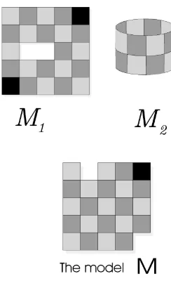
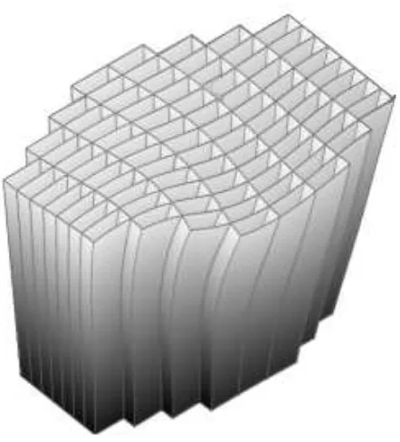
(or any manifold). The second one, based on an example in the article [We4], is a bit more fanciful-a sort of “toy pseudogroup”. Consider the object labelled “The modelM” in figure 2.1. Consider this set as made of tiles and their edges (grout between the tiles plus the outer boundary). Let Γ be the set of all maps from open sets of the plane to open sets of the plane that are restrictions of rigid motions of the plane. The we take as our example Γtoy := Γ|M which is

the homeomorphisms of (relatively) open sets ofMto open sets ofMwhich are restrictions of the maps in Γ (to the intersections of their domains withM).

Definition 2.4 Apseudogroup of transformations, sayΓ, of a topological spaceX is a family_{Φγ}γ∈I of homeomorphisms with domainUγ and rangeVγ

both open subsets of X, which satisfies the following properties: 1) idX∈Γ.

2)Φγ ∈Γ impliesΦ−γ1∈Γ.

3) For any open setU _⊂X, the restrictions Φγ|U are inΓ for all Φγ ∈Γ.

4) The composition of any two elements Φγ, Φν ∈ Γ are elements of Γ

whenever the composition is defined:

(33)

2.4. PSEUDO-GROUPS AND MODELS SPACES 23

Figure 2.1: Tile and grout spaces

5) For any subfamily{Φγ}γ∈G1 ⊂Γ such that Φγ|U_γ_∩Uν = Φν|Uγ∩Uν

when-ever Uγ∩Uν 6=∅ then the mapping defined byΦ :Sγ∈G1Uγ → S

γ∈G1Vγ is an

element ofΓ if it is a homeomorphism.

Exercise 2.2 Check that each of these axioms is satisfied by our “fanciful ex-ample” Γtoy.

Definition 2.5 Asub-pseudogroup Σof a pseudogroup is a subset of Γ that is also a pseudogroup (and so closed under composition and inverses).

We will be mainly interested inCr_{-pseudogroups and the spaces which}

sup-port them. Our main example will be the set Γr

Rn of all Cr diffeomorphisms

between open subsets ofRn_{. More generally, for a Banach space}_B_{we have the}

Cr_{-pseudo-group Γ}r

B consisting of all Crdiffeomorphisms between open subsets

of a Banach spaceB. Since this is our prototype the reader should spend some time thinking about this example.

Definition 2.6 ACr

−pseudogroupΓof transformations of a subsetMof Ba-nach space B is a pseudogroup arising as the restriction to M of some sub-pseudogroup of Γr

M. The pair (M,Γ) is called a model space . As is usual in

cases like this we sometimes just refer toM as the model space.

Example 2.8 Recall that a mapU ⊂Cn _→_Cn_{is holomorphic if the derivative}

(from the point of view of the underlying real spaceR2n_{) is in fact complex linear.}

Mathematics Differential Geometry Analysis and Physics

Differential Geometry, Analysis and Physics

Jeffrey M. Lee

c

Contents

0.1

Preface

Chapter 1

Preliminaries and Local

Theory

1.1

Calculus

§§

Interlude

§§

Infinite dimensions.

§§

§

Interlude

§

Thinking about derivatives in infinite dimensions

1.2

Chain Rule, Product rule and Taylor’s

The-orem

1.3

Local theory of maps

Chapter 2

Differentiable Manifolds

2.1

Rough Ideas I

2.2

Topological Manifolds

2.3

Differentiable Manifolds and Differentiable

Maps

2.4

Pseudo-Groups and Models Spaces