Database Anonymization
Privacy Models, Data Utility, and
Microaggregation-based
Inter-model Connections
Josep Domingo-Ferrer
David Sánchez
Jordi Soria-Comas
Elisa Bertino & Ravi Sandhu,
Series Editors
M OR G A N
&
C L AY P O OL P U B L I S H E R S
S
YNTHESIS
L
ECTURES
ON
Database Anonymization
Synthesis Lectures on
Information Security, Privacy,
& Trust
Editor
Elisa Bertino,Purdue University
Ravi Sandhu,University of Texas at San Antonio
e Synthesis Lectures Series on Information Security, Privacy, and Trust publishes 50- to 100-page publications on topics pertaining to all aspects of the theory and practice of Information Security, Privacy, and Trust. e scope largely follows the purview of premier computer security research journals such as ACM Transactions on Information and System Security, IEEE Transactions on Dependable and Secure Computing and Journal of Cryptology, and premier research conferences, such as ACM CCS, ACM SACMAT, ACM AsiaCCS, ACM CODASPY, IEEE Security and Privacy, IEEE Computer Security Foundations, ACSAC, ESORICS, Crypto, EuroCrypt and AsiaCrypt. In addition to the research topics typically covered in such journals and conferences, the series also solicits lectures on legal, policy, social, business, and economic issues addressed to a technical audience of scientists and engineers. Lectures on significant industry developments by leading practitioners are also solicited.
Database Anonymization: Privacy Models, Data Utility, and Microaggregation-based Inter-model Connections
Josep Domingo-Ferrer, David Sánchez, and Jordi Soria-Comas 2016
Automated Software Diversity
Per Larsen, Stefan Brunthaler, Lucas Davi, Ahmad-Reza Sadeghi, and Michael Franz 2015
Trust in Social Media No Access Jiliang Tang and Huan Liu
2015
Physically Unclonable Functions (PUFs): Applications, Models, and Future Directions No Access
iii
Usable Security: History, emes, and Challenges No Access Simson Garfinkel and Heather Richter Lipford
2014
Reversible Digital Watermarking: eory and Practices No Access Ruchira Naskar and Rajat Subhra Chakraborty
2014
Mobile Platform Security No Access
N. Asokan, Lucas Davi, Alexandra Dmitrienko, Stephan Heuser, Kari Kostiainen, Elena Reshetova, and Ahmad-Reza Sadeghi
2013
Security and Trust in Online Social Networks No Access Barbara Carminati, Elena Ferrari, and Marco Viviani
2013
RFID Security and Privacy No Access Yingjiu Li, Robert H. Deng, and Elisa Bertino 2013
Hardware Malware No Access
Christian Krieg, Adrian Dabrowski, Heidelinde Hobel, Katharina Krombholz, and Edgar Weippl 2013
Private Information Retrieval No Access Xun Yi, Russell Paulet, and Elisa Bertino 2013
Privacy for Location-based Services No Access Gabriel Ghinita
2013
Enhancing Information Security and Privacy by Combining Biometrics with Cryptography No Access
Sanjay G. Kanade, Dijana Petrovska-Delacrétaz, and Bernadette Dorizzi 2012
Analysis Techniques for Information Security No Access
Anupam Datta, Somesh Jha, Ninghui Li, David Melski, and omas Reps 2010
Operating System Security No Access Trent Jaeger
All rights reserved. No part of this publication may be reproduced, stored in a retrieval system, or transmitted in any form or by any means—electronic, mechanical, photocopy, recording, or any other except for brief quotations in printed reviews, without the prior permission of the publisher.
Database Anonymization:
Privacy Models, Data Utility, and Microaggregation-based Inter-model Connections Josep Domingo-Ferrer, David Sánchez, and Jordi Soria-Comas
www.morganclaypool.com
ISBN: 9781627058438 paperback ISBN: 9781627058445 ebook
DOI 10.2200/S00690ED1V01Y201512SPT015
A Publication in the Morgan & Claypool Publishers series
SYNTHESIS LECTURES ON INFORMATION SECURITY, PRIVACY, & TRUST
Lecture #15
Series Editors: Elisa Bertino,Purdue University
Ravi Sandhu,University of Texas at San Antonio Series ISSN
Database Anonymization
Privacy Models, Data Utility, and Microaggregation-based
Inter-model Connections
Josep Domingo-Ferrer, David Sánchez, and Jordi Soria-Comas
Universitat Rovira i Virgili, Tarragona, CataloniaSYNTHESIS LECTURES ON INFORMATION SECURITY, PRIVACY, &
TRUST #15
C
M
ABSTRACT
e current social and economic context increasingly demands open data to improve scientific research and decision making. However, when published data refer to individual respondents, disclosure risk limitation techniques must be implemented to anonymize the data and guaran-tee by design the fundamental right to privacy of the subjects the data refer to. Disclosure risk limitation has a long record in the statistical and computer science research communities, who have developed a variety of privacy-preserving solutions for data releases. is Synthesis Lec-ture provides a comprehensive overview of the fundamentals of privacy in data releases focusing on the computer science perspective. Specifically, we detail the privacy models, anonymization methods, and utility and risk metrics that have been proposed so far in the literature. Besides, as a more advanced topic, we identify and discuss in detail connections between several privacy models (i.e., how to accumulate the privacy guarantees they offer to achieve more robust pro-tection and when such guarantees are equivalent or complementary); we also explore the links between anonymization methods and privacy models (how anonymization methods can be used to enforce privacy models and thereby offerex anteprivacy guarantees). ese latter topics are relevant to researchers and advanced practitioners, who will gain a deeper understanding on the available data anonymization solutions and the privacy guarantees they can offer.
KEYWORDS
vii
A tots aquells que estimem, tant si són amb nosaltres
com si perviuen en el nostre record.
ix
Contents
Preface. . . .xiii
Acknowledgments. . . xv
1
Introduction . . . 12
Privacy in Data Releases. . . 32.1 Types of Data Releases . . . 4
2.2 Microdata Sets . . . 4
2.3 Formalizing Privacy . . . 6
2.4 Disclosure Risk in Microdata Sets . . . 8
2.5 Microdata Anonymization . . . 9
2.6 Measuring Information Loss . . . 10
2.7 Trading Off Information Loss and Disclosure Risk . . . 12
2.8 Summary . . . 13
3
Anonymization Methods for Microdata . . . 153.1 Non-perturbative Masking Methods . . . 15
3.2 Perturbative Masking Methods . . . 16
3.3 Synthetic Data Generation . . . 21
3.4 Summary . . . 22
4
Quantifying Disclosure Risk: Record Linkage. . . 254.1 reshold-based Record Linkage. . . 26
4.2 Rule-based Record Linkage . . . 26
4.3 Probabilistic Record Linkage . . . 27
4.4 Summary . . . 29
5
ek-Anonymity Privacy Model. . . 315.1 Insufficiency of Data De-identification . . . 31
5.2 ek-Anonymity Model . . . 33
5.4 Microaggregation-basedk-Anonymity . . . 42
5.5 Probabilistick-Anonymity . . . 43
5.6 Summary . . . 44
6
Beyondk-Anonymity:l-Diversity andt-Closeness. . . 476.1 l-Diversity . . . 47
6.2 t-Closeness . . . 48
6.3 Summary . . . 51
7
t-Closeness rough Microaggregation . . . 537.1 Standard Microaggregation and Merging . . . 53
7.2 t-Closeness Aware Microaggregation:k-anonymity-first . . . 55
7.3 t-Closeness Aware Microaggregation:t-closeness-first . . . 55
7.4 Summary . . . 62
8
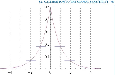
Differential Privacy. . . 658.1 Definition . . . 65
8.2 Calibration to the Global Sensitivity . . . 66
8.3 Calibration to the Smooth Sensitivity . . . 70
8.4 e Exponential Mechanism . . . 72
8.5 Relation tok-anonymity-based Models . . . 73
8.6 Differentially Private Data Publishing . . . 75
8.7 Summary . . . 77
9
Differential Privacy by Multivariate Microaggregation. . . 799.1 Reducing Sensitivity Via Prior Multivariate Microaggregation . . . 79
9.2 Differentially Private Data Sets by Insensitive Microaggregation . . . 85
9.3 General Insensitive Microaggregation . . . 87
9.4 Differential Privacy with Categorical Attributes . . . 88
9.5 A Semantic Distance for Differential Privacy . . . 92
9.6 Integrating Heterogeneous Attribute Types . . . 94
9.7 Summary . . . 94
10
Differential Privacy by Individual Ranking Microaggregation. . . 9710.1 Limitations of Multivariate Microaggregation . . . 97
xi
10.3 Choosing the Microggregation Parameterk . . . 102
10.4 Summary . . . 102
11
Conclusions and Research Directions. . . 10511.1 Summary and Conclusions . . . 105
11.2 Research Directions . . . 106
Bibliography . . . 109
xiii
Preface
If jet airplanes ushered in the first dramatic reduction of our world’s perceived size, the next shrinking came in the mid 1990s, when the Internet became widespread and the Information Age started to become a reality. We now live in a global village and some (often quite powerful) voices proclaim that maintaining one’s privacy is as hopeless as it used to be in conventional small villages. Should this be true, the ingenuity of humans would have created their own nightmare.
Whereas security is essential for organizations to survive, individuals and sometimes even companies need also some privacy to develop comfortably and lead a free life. is is the reason individual privacy is mentioned in the Universal Declaration of Human Rights (1948) and data privacy is protected by law in most Western countries. Indeed, without privacy, other fundamental rights, like freedom of speech and democracy, are impaired. e outstanding challenge is to create technology that implements those legal guarantees in a way compatible with functionality and security.
is book is devoted to privacy preservation in data releases. Indeed, in our era of big data, harnessing the enormous wealth of information available is essential to increasing the progress and well-being of humankind. e challenge is how to release data that are useful for administrations and companies to make accurate decisions without disclosing sensitive information on specific identifiable individuals.
is conflict between utility and privacy has motivated research by several communities since the 1970s, both in official statistics and computer science. Specifically, computer scientists contributed the important notion of the privacy model in the late 1990s, withk-anonymity being the first practical privacy model. e idea of a privacy model is to stateex anteprivacy guarantees that can be attained for a particular data set using one (or several) anonymization methods.
We sincerely hope that the reader, whether academic or practitioner, will benefit from this piece of work. On our side, we have enjoyed writing it and also conducting the original research described in some of the chapters.
xv
Acknowledgments
We thank Professor Elisa Bertino for encouraging us to write this Synthesis Lecture. is work was partly supported by the European Commission (through project H2020 “CLARUS”), by the Spanish Government (through projects “ICWT” TIN2012-32757 and “SmartGlacis” TIN2014-57364-C2-1-R), by the Government of Catalonia (under grant 2014 SGR 537), and by the Tem-pleton World Charity Foundation (under project “CO-UTILITY”). Josep Domingo-Ferrer is partially supported as an ICREA-Acadèmia researcher by the Government of Catalonia. e au-thors are with the UNESCO Chair in Data Privacy, but the opinions expressed in this work are the authors’ own and do not necessarily reflect the views of UNESCO or any of the funders.
1
C H A P T E R 1
Introduction
e current social and economic context increasingly demands open data to improve planning, scientific research, market analysis, etc. In particular, the public sector is pushed to release as much information as possible for the sake of transparency. Organizations releasing data include national statistical institutes (whose core mission is to publish statistical information), healthcare authorities (which occasionally release epidemiologic information) or even private organizations (which sometimes publish consumer surveys). When published data refer to individual respon-dents, care must be exerted for the privacy of the latter not to be violated. It should bede facto
impossible to relate the published data to specific individuals. Indeed, supplying data to national statistical institutes is compulsory in most countries but, in return, these institutes commit to pre-serving the privacy of the respondents. Hence, rather than publishing accurate information for each individual, the aim should be to provide useful statistical information, that is, to preserve as much as possible in the released data the statistical properties of the original data.
Disclosure risk limitation has a long tradition in official statistics, where privacy-preserving databases on individuals are calledstatistical databases. Inference control in statistical databases, also known asStatistical Disclosure Control (SDC),Statistical Disclosure Limitation (SDL),database anonymization, ordatabase sanitization, is a discipline that seeks to protect data so that they can be published without revealing confidential information that can be linked to specific individuals among those to whom the data correspond.
Disclosure limitation has also been a topic of interest in the computer science research com-munity, which refers to it asPrivacy Preserving Data Publishing (PPDP)andPrivacy Preserving Data Mining (PPDM). e latter focuses on protecting the privacy of the results of data mining tasks, whereas the former focuses on the publication of data of individuals.
Whereas both SDC and PPDP pursue the same objective, SDC proposes protection mech-anisms that are more concerned with the utility of the data and offer only vague (i.e.,ex post) privacy guarantees, whereas PPDP seeks to attain anex anteprivacy guarantee (by adhering to a privacy model), but offers no utility guarantees.
privacy models (i.e., how specific SDC methods can be used to satisfy specific privacy models and thereby offerex anteprivacy guarantees).
e book is organized as follows.
• Chapter2details the basic notions of privacy in data releases: types of data releases, privacy threats and metrics, and families of SDC methods.
• Chapter3offers a comprehensive overview of SDC methods, classified into perturbative and non-perturbative ones.
• Chapter4describes how disclosure risk can be empirically quantified via record linkage. • Chapter5discusses the well-knownk-anonymity privacy model, which is focused on
pre-venting re-identification of individuals, and details which data protection mechanisms can be used to enforce it.
• Chapter6 describes two extensions ofk-anonymity (l-diversity andt-closeness) focused on offering protection against attribute disclosure.
• Chapter 7 presents in detail how t-closeness can be attained on top ofk-anonymity by relying on data microaggregation (i.e., a specific SDC method based on data clustering). • Chapter8describes the differential privacy model, which mainly focuses on providing
sani-tized answers with robust privacy guarantees to specific queries. We also explain SDC tech-niques that can be used to attain differential privacy. We also discuss in detail the relation-ship between differential privacy andk-anonymity-based models (t-closeness, specifically). • Chapters9and10present two state-of-the-art approaches to offer utility-preserving dif-ferentially private data releases by relying on the notion ofk-anonymous data releases and on multivariate and univariate microaggregation, respectively.
3
C H A P T E R 2
Privacy in Data Releases
References to privacy were already present in the writings of Greek philosophers when they dis-tinguish theouter(public) from theinner(private). Nowadays privacy is considered a fundamental right of individuals [34,101]. Despite this long history, the formal description of the “right to privacy” is quite recent. It was coined by Warren and Brandeis, back in 1890, in an article [103] published in theHarvard Law Review. ese authors presented laws as dynamic systems for the protection of individuals whose evolution is triggered by social, political, and economic changes. In particular, the conception of the right to privacy is triggered by the technical advances and new business models of the time. Quoting Warren and Brandeis:
Instantaneous photographs and newspaper enterprise have invaded the sacred precincts of private and domestic life; and numerous mechanical devices threaten to make good the prediction that what is whispered in the closet shall be proclaimed from the house-tops.
Warren and Brandeis argue that the “right to privacy” was already existent in many areas of the common law; they only gathered all these sparse legal concepts, and put them into focus under their common denominator. Within the legal framework of the time, the “right to privacy” was part of the right to life, one of the three fundamental individual rights recognized by the U.S. constitution.
Privacy concerns revived again with the invention of computers [31] and information ex-change networks, which skyrocketed information collection, storage and processing capabilities. e generalization of population surveys was a consequence. e focus was then on data protec-tion.
Nowadays, privacy is widely considered a fundamental right, and it is supported by inter-national treaties and many constitutional laws. For example, the Universal Declaration of Human Rights (1948) devotes its Article 12 to privacy. In fact, privacy has gained worldwide recognition and it applies to a wide range of situations such as: avoiding external meddling at home, limiting the use of surveillance technologies, controlling processing and dissemination of personal data, etc.
Among all the aspects that relate to data privacy, we are especially interested in data dissem-ination. Dissemination is, for instance, the primary task of National Statistical Institutes. ese aim at offering an accurate picture of society; to that end, they collect and publish statistical data on a wide range of aspects such as economy, population, etc. Legislation usually assimilates pri-vacy violations in data dissemination to individual identifiability [1, 2]; for instance, Title 13, Chapter 1.1 of the U.S. Code states that “no individual should be re-identifiable in the released data.”
For a more comprehensive review of the history of privacy, check [43]. A more visual per-spective of privacy is given by the timelines [3,4]. In [3] key privacy-related events between 1600 (when it was a civic duty to keep an eye on your neighbors) and 2008 (after the U.S. Patriot Act and the inception of Facebook) are listed. In [4] key moments that have shaped privacy-related laws are depicted.
2.1 TYPES OF DATA RELEASES
e type of data being released determines the potential threats to privacy as well as the most suitable protection methods. Statistical databases come in three main formats.
• Microdata. e term “microdata” refers to a record that contains information related to a specific individual (a citizen or a company). A microdata release aims at publishing raw data, that is, a set of microdata records.
• Tabular data. Cross-tabulated values showing aggregate values for groups of individuals are released. e term contingency (or frequency) table is used when counts are released, and the term “magnitude table” is used for other aggregate magnitudes. ese types of data is the classical output of official statistics.
• Queryable databases, that is, interactive databases to which the user can submit statistical queries (sums, averages, etc.).
Our focus in subsequent chapters is on microdata releases. Microdata offer the greatest level of flexibility among all types of data releases: data users are not confined to a specific prefixed view of data; they are able to carry out any kind of custom analysis on the released data. However, microdata releases are also the most challenging for the privacy of individuals.
2.2 MICRODATA SETS
2.2. MICRODATA SETS 5
e attributes in a microdata set are usually classified in the following non-exclusive cate-gories.
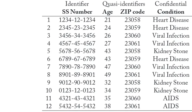
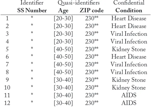
• Identifiers.An attribute is an identifier if it provides unambiguous re-identification of the individual to which the record refers. Some examples of identifier attributes are the social security number, the passport number, etc. If a record contains an identifier, any sensitive information contained in other attributes may immediately be linked to a specific individual. To avoid direct re-identification of an individual, identifier attributes must be removed or encrypted. In the following chapters, we assume that identifier attributes have previously been removed.
• Quasi-identifiers. Unlike an identifier, a quasi-identifier attribute alone does not lead to record re-identification. However, in combination with other quasi-identifier attributes, it may allow unambiguous re-identification of some individuals. For example, [99] shows that 87% of the population in the U.S. can be unambiguously identified by combining a 5-digit ZIP code, birth date, and sex. Removing quasi-identifier attributes, as proposed for the identifiers, is not possible, because quasi-identifiers are most of the time required to perform any useful analysis of the data. Deciding whether a specific attribute should be considered a quasi-identifier is a thorny issue. In practice, any information an intruder has about an individual can be used in record re-identification. For uninformed intruders, only the attributes available in an external non-anonymized data set should be classified as quasi-identifiers; in the presence of informed intruders any attribute may potentially be a quasi-identifier. us, in the strictest case, to make sure all potential quasi-identifiers have been removed, one ought to remove all attributes (!).
• Confidential attributes.Confidential attributes hold sensitive information on the individuals that took part in the data collection process (e.g., salary, health condition, sex orientation, etc.). e primary goal of microdata protection techniques is to prevent intruders from learning confidential information about a specific individual. is goal involves not only preventing the intruder from determining the exact value that a confidential attribute takes for some individual, but also preventing accurate inferences on the value of that attribute (such as bounding it).
2.3 FORMALIZING PRIVACY
A first attempt to come up with a formal definition of privacy was made by Dalenius in [14]. He stated that access to the released data should not allow any attacker to increase his knowledge about confidential information related to a specific individual. In other words, the prior and the posterior beliefs about an individual in the database should be similar. Because the ultimate goal in privacy is to keep the secrecy of sensitive information about specific individuals, this is a natural definition of privacy. However, Dalenius’ definition is too strict to be useful in practice. is was illustrated with two examples [29]. e first one considers an adversary whose prior view is that everyone has two left feet. By accessing a statistical database, the adversary learns that almost everybody has one left foot and one right foot, thus modifying his posterior belief about individuals to a great extent. In the second example, the use of auxiliary information makes things worse. Suppose that a statistical database teaches the average height of a group of individuals, and that it is not possible to learn this information in any other way. Suppose also that the actual height of a person is considered to be a sensitive piece of information. Let the attacker have the following side information: “Adam is one centimeter taller than the average English man.” Access to the database teaches Adam’s height, while having the side information but no database access teaches much less. us, Dalenius’ view of privacy is not feasible in presence of background information (if any utility is to be provided).
e privacy criteria used in practice offer only limited disclosure control guarantees. Two main views of privacy are used for microdata releases: anonymity (it should not be possible to re-identify any individual in the published data) and confidentiality or secrecy (access to the released data should not reveal confidential information related to any specific individual).
e confidentiality view of privacy is closer to Dalenius’ proposal, being the main difference that it limits the amount of information provided by the data set rather than the change between prior and posterior beliefs about an individual. ere are several approaches to attain confiden-tiality. A basic example of SDC technique that gives confidentiality is noise addition. By adding a random noise to a confidential data item, we mask its value: we report a value drawn from a random distribution rather than the actual value. e amount of noise added determines the level of confidentiality.
2.3. FORMALIZING PRIVACY 7
e Health Insurance Portability and Accountability Act (HIPAA)
e Privacy Rule allows a covered entity to de-identify data by removing all 18 ele-ments that could be used to identify the individual or the individual’s relatives, employers, or household members; these elements are enumerated in the Privacy Rule. e covered entity also must have no actual knowledge that the remaining information could be used alone or in combination with other information to identify the individual who is the subject of the information. Under this method, the identifiers that must be removed are the following:
• Names.
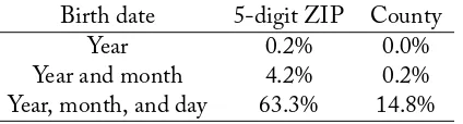
• All geographic subdivisions smaller than a state, including street address, city, county, precinct, ZIP code, and their equivalent geographical codes, except for the initial three digits of a ZIP code if, according to the current publicly available data from the Bureau of the Census:
– e geographic unit formed by combining all ZIP codes with the same three initial digits contains more than 20,000 people.
– e initial three digits of a ZIP code for all such geographic units containing 20,000 or fewer people are changed to 000.
• All elements of dates (except year) for dates directly related to an individual, including birth date, admission date, discharge date, date of death; and all ages over 89 and all elements of dates (including year) indicative of such age, except that such ages and elements may be aggregated into a single category of age 90 or older.
• Telephone numbers. • Facsimile numbers. • Electronic mail addresses. • Social security numbers. • Medical record numbers.
• Health plan beneficiary numbers. • Account numbers.
• Certificate/license numbers.
• Web universal resource locators (URLs). • Internet protocol (IP) address numbers.
• Biometric identifiers, including fingerprints and voiceprints. • Full-face photographic images and any comparable images.
• Any other unique identifying number, characteristic, or code, unless otherwise permit-ted by the Privacy Rule for re-identification.
2.4 DISCLOSURE RISK IN MICRODATA SETS
When publishing a microdata file, the data collector must guarantee that no sensitive information about specific individuals is disclosed. Usually two types of disclosure are considered in microdata sets [44].
• Identity disclosure. is type of disclosure violates privacy viewed as anonymity. It occurs when the intruder is able to associate a record in the released data set with the individual that originated it. After re-identification, the intruder associates the values of the confidential attributes for the record to the re-identified individual. Two main approaches are usually employed to measure identity disclosure risk: uniqueness and reidentification.
– Uniqueness. Roughly speaking, the risk of identity disclosure is measured as the prob-ability that rare combinations of attribute values in the released protected data are indeed rare in the original population the data come from.
– Record linkage. is is an empirical approach to evaluate the risk of disclosure. In this case, the data protector (also known as data controller) uses a record linkage algo-rithm (or several such algoalgo-rithms) to link each record in the anonymized data with a record in the original data set. Since the protector knows the real correspondence be-tween original and anonymized records, he can determine the percentage of correctly linked pairs, which he uses to estimate the number of re-identifications that might be obtained by a specialized intruder. If this number is unacceptably high, then more intense anonymization by the controller is needed before the anonymized data set is ready for release.
• Attribute disclosure. is type of disclosure violates privacy viewed as confidentiality. It occurs when access to the released data allows the intruder to determine the value of a confidential attribute of an individual with enough accuracy.
2.5. MICRODATA ANONYMIZATION 9
masked. On the other side, attribute disclosure may still happen even without identity disclosure. For example, imagine that the salary is one of the confidential attributes and the job is a quasi-identifier attribute; if an intruder is interested in a specific individual whose job he knows to be “accountant” and there are several accountants in the data set (including the target individual), the intruder will be unable to re-identify the individual’s record based only on her job, but he will be able to lower-bound and upper-bound the individual’s salary (which lies between the minimum and the maximum salary of all the accountants in the data set). Specifically, attribute disclosure happens if the range of possible salary values for the matching records is narrow.
2.5 MICRODATA ANONYMIZATION
To avoid disclosure, data collectors do not publish the original microdata setX, but a modified versionY of it. is data setY is called the protected, anonymized, or sanitized version ofX. Microdata protection methods can generate the protected data set by either masking the original data or generating synthetic data.
• Masking. e protected dataY are generated by modifying the original records inX. Mask-ing induces a relation between the records inY and the original records inX. When ap-plied to quasi-identifier attributes, the identity behind each record is masked (which yields anonymity). When applied to confidential attributes, the values of the confidential data are masked (which yields confidentiality, even if the subject to whom the record corresponds might still be re-identifiable). Masking methods can in turn be divided in two categories depending on their effect on the original data.
– Perturbative masking. e microdata set is distorted before publication. e perturba-tion method used should be such that the statistics computed on the perturbed data set do not differ significantly from the statistics that would be obtained on the original data set. Noise addition, microaggregation, data/rank swapping, microdata rounding, resampling, and PRAM are examples of perturbative masking methods.
– Non-perturbative masking. Non-perturbative methods do not alter data; rather, they produce partial suppressions or reductions of detail/coarsening in the original data set. Sampling, global recoding, top and bottom coding, and local suppression are examples of non-perturbative masking methods.
– Fully synthetic[77], where every attribute value for every record has been synthesized. e population units (subjects) contained inY are not the original population units in Xbut a new sample from the underlying population.
– Partially synthetic[74], where only the data items (the attribute values) with high risk of disclosure are synthesized. e population units inY are the same population units inX(in particular,X andY have the same number of records).
– Hybrid[19,65], where the original data set is mixed with a fully synthetic data set. In a fully synthetic data set any dependency betweenXandY must come from the model. In other words,X and Y are independent conditionally to the adjusted model. e dis-closure risk in fully synthetic data sets is usually low, as we justify next. On the one side, the population units inY are not the original population units in X. On the other side, the information about the original dataX conveyed byY is only the one incorporated by the model, which is usually limited to some statistical properties. In a partially synthetic data set, the disclosure risk is reduced by replacing the values in the original data set at a higher risk of disclosure with simulated values. e simulated values assigned to an indi-vidual should be representative but are not directly related to her. In hybrid data sets, the level of protection we get is the lowest; mixing original and synthetic records breaks the conditional independence between the original data and the synthetic data. e parameters of the mixture determine the amount of dependence.
2.6 MEASURING INFORMATION LOSS
e evaluation of the utility of the protected data set must be based on the intended uses of the data. e closer the results obtained for these uses between the original and the protected data, the more utility is preserved. However, very often, microdata protection cannot be performed in a data use specific manner, due to the following reasons.
• Potential data uses are very diverse and it may even be hard to identify them all at the moment of the data release.
• Even if all the data uses could be identified, releasing several versions of the same original data set so that the i-th version has been optimized for the i-th data use may result in unexpected disclosure.
Since data must often be protected with no specific use in mind, it is usually more appropriate to refer to information loss rather than to utility. Measures of information loss provide generic ways for the data protector to assess how much harm is being inflicted to the data by a particular data masking technique.
2.6. MEASURING INFORMATION LOSS 11
• Covariance matricesV (onX) andV0(onY). • Correlation matricesRandR0.
• Correlation matrices RF and RF0 between the m attributes and the m factors P C1; P C2; : : : ; P Cpobtained through principal components analysis.
• Communality between each of the mattributes and the first principal component P C1 (or other principal componentsP Ci’s). Communality is the percent of each attribute that is explained byP C1 (orP Ci). LetC be the vector of communalities forX, andC0 the corresponding vector forY.
• Factor score coefficient matricesF andF0. MatrixF contains the factors that should mul-tiply each attribute in X to obtain its projection on each principal component. F0 is the corresponding matrix forY.
ere does not seem to be a single quantitative measure which completely reflects the structural differences betweenX andY. erefore, in [25,87] it was proposed to measure the information loss through the discrepancies between matricesX,V,R,RF,C, andF obtained on the original data and the correspondingX0,V0,R0,RF0,C0, andF0 obtained on the protected data set. In particular, discrepancy between correlations is related to the information loss for data uses such as regressions and cross-tabulations. Matrix discrepancy can be measured in at least three ways.
• Mean square error.Sum of squared componentwise differences between pairs of matrices, divided by the number of cells in either matrix.
• Mean absolute error.Sum of absolute componentwise differences between pairs of matrices, divided by the number of cells in either matrix.
• Mean variation.Sum of absolute percent variation of components in the matrix computed on the protected data with respect to components in the matrix computed on the original data, divided by the number of cells in either matrix. is approach has the advantage of not being affected by scale changes of attributes.
Information loss measures for categorical data. ese have been usually based on direct compari-son of categorical values, comparicompari-son of contingency tables, or on Shannon’s entropy [25]. More recently, the importance of the semantics underlying categorical data for data utility has been realized [60,83]. As a result, semantically grounded information loss measures that exploits the formal semantics provided by structured knowledge sources (such as taxonomies or ontologies) have been proposed both to measure the practical utility and to guide the sanitization algorithms in terms of the preservation of data semantics [23,57,59].
between 0 and 1). Defining bounded information loss measures may be convenient to enable the data protector to trade off information loss against disclosure risk. In [61], probabilistic informa-tion loss measures bounded between 0 and 1 are proposed for continuous data.
Propensity scores: a global information loss measure for all types of data. In [105], an infor-mation loss measureU applicable to continuous and categorical microdata was proposed. It is computed as follows.
1. Merge the original microdata setX and the anonymized microdata setY, and add to the merged data set a binary attributeT with value 1 for the anonymized records and 0 for the original records.
2. RegressT on the rest of attributes of the merged data set and call the adjusted attributeTO. For categorical attributes, logistic regression can be used.
3. Let thepropensity scorepiO of recordi of the merged data set be the value ofTO for recordi. en the utility ofY is high if the propensity scores of the anonymized and original records are similar (this means that, based on the regression model used, anonymized records cannot be distinguished from original records).
4. Hence, if the number of original and anonymized records is the same, sayN, a utility mea-sure is
e fartherU from 0, the more information loss, and conversely.
2.7 TRADING OFF INFORMATION LOSS AND
DISCLOSURE RISK
e goal of SDC to modify data so that sufficient protection is provided at minimum information loss suggests that a good anonymization method is one close to optimizing the trade-off between disclosure risk and information loss. Several approaches have been proposed to handle this trade-off. Here we discuss SDC scores and R-U maps.
SDC scores
An SDC score is a formula that combines the effects of information loss and disclosure risk in a single figure. Having adopted an SDC score as a good trade-off measure, the goal is to optimize the score value. Following this idea, [25] proposed a score for method performance rating based on the average of information loss and disclosure risk measures. For each methodM and parameterizationP, the following score is computed:
ScoreM;P.X; Y /D
2.8. SUMMARY 13
where IL is an information loss measure, DR is a disclosure risk measure, and Y is the pro-tected data set obtained after applying methodM with parameterizationP to an original data setX. In [25]ILandDRwere computed using a weighted combination of several information
loss and disclosure risk measures. With the resulting score, a ranking of masking methods (and their parametrizations) was obtained. Using a score permits regarding the selection of a masking method and its parameters as an optimization problem: a masking method can be applied to the original data file and then a post-masking optimization procedure can be applied to decrease the score obtained (that is, to reduce information loss and disclosure risk). On the negative side, no specific score weighting can do justice to all methods. us, when ranking methods, the values of all measures of information loss and disclosure risk should be supplied along with the overall score.
R-U maps
A tool which may be enlightening when trying to construct a score or, more generally, optimize the trade-off between information loss and disclosure risk is a graphical representation of pairs of measures (disclosure risk, information loss) or their equivalents (disclosure risk, data utility). Such maps are called R-U confidentiality maps [28]. Here, R stands for disclosure risk and U for data utility. In its most basic form, an R-U confidentiality map is the set of paired values (R,U) of disclosure risk and data utility that correspond to the various strategies for data release (e.g., variations on a parameter). Such (R,U) pairs are typically plotted in a two-dimensional graph, so that the user can easily grasp the influence of a particular method and/or parameter choice.
2.8 SUMMARY
15
C H A P T E R 3
Anonymization Methods for
Microdata
It was commented in Section2.5that the protected data setY was generated either by masking the original data set X or by building it from scratch based on a model of the original data. Microdata masking techniques were further classified into perturbative masking (which distorts the original data and leads to the publication of non-truthful data) and non-perturbative masking (which reduces the amount of information, either by suppressing some of the data or by reducing the level of detail, but preserves truthfulness). is chapter classifies and reviews some well-known SDC techniques. ese techniques are not only useful on their own but they also constitute the basis to enforce the privacy guarantees required by privacy models.
3.1 NON-PERTURBATIVE MASKING METHODS
Non-perturbative methods do not alter data; rather, they produce partial suppressions or reduc-tions of detail in the original data set.
Sampling
Instead of publishing the original microdata fileX, what is published is a sampleSof the original set of records [104]. Sampling methods are suitable for categorical microdata [58], but for con-tinuous microdata they should probably be combined with other masking methods. e reason is that sampling alone leaves a continuous attribute unperturbed for all records inS. us, if any continuous attribute is present in an external administrative public file, unique matches with the published sample are very likely: indeed, given a continuous attribute and two respondentsxi andxj, it is unlikely that both respondents will take the same value for the continuous attribute unlessxi Dxj(this is true even if the continuous attribute has been truncated to represent it dig-itally). If, for a continuous identifying attribute, the score of a respondent is only approximately known by an attacker, it might still make sense to use sampling methods to protect that attribute. However, assumptions on restricted attacker resources are perilous and may prove definitely too optimistic if good quality external administrative files are at hand.
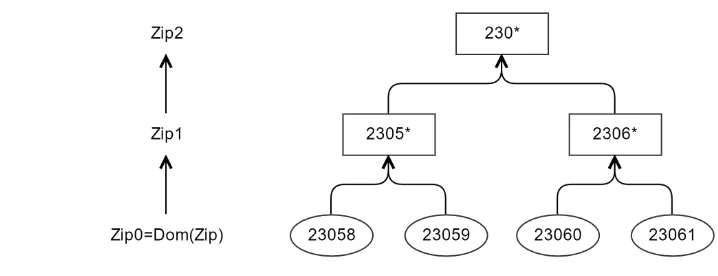
Generalization
thus resulting in a newYi with jDom.Yi/j<jDom.Xi/j wherej·j is the cardinality operator
andDom.·/is the domain where the attribute takes values. For a continuous attribute, general-ization means replacingXiby another attributeYiwhich is a discretized version ofXi. In other words, a potentially infinite rangeDom.Xi/ is mapped onto a finite range Dom.Yi/. is is the technique used in the-Argus SDC package [45]. is technique is more appropriate for categorical microdata, where it helps disguise records with strange combinations of categorical attributes. Generalization is used heavily by statistical offices.
Example3.1 If there is a record with “Marital status = Widow/er” and “Age = 17,” generalization could be applied to “Marital status” to create a broader category “Widow/er or divorced,” so that the probability of the above record being unique would diminish. Generalization can also be used on a continuous attribute, but the inherent discretization leads very often to an unaffordable loss of information. Also, arithmetical operations that were straightforward on the originalXiare no longer easy or intuitive on the discretizedYi.
Top and bottom coding
Top and bottom coding are special cases of generalization which can be used on attributes that can be ranked, that is, continuous or categorical ordinal. e idea is that top values (those above a certain threshold) are lumped together to form a new category. e same is done for bottom values (those below a certain threshold).
Local suppression
is is a masking method in which certain values of individual attributes are suppressed with the aim of increasing the set of records agreeing on a combination of key values. Ways to combine local suppression and generalization are implemented in the-Argus SDC package [45].
If a continuous attributeXi is part of a set of key attributes, then each combination of key values is probably unique. Since it does not make sense to systematically suppress the values of Xi, we conclude that local suppression is rather oriented to categorical attributes.
3.2 PERTURBATIVE MASKING METHODS
Noise addition
Additive noise is a family of perturbative masking methods. e values in the original data set are masked by adding some random noise. e statistical properties of the noise being added determine the effect of noise addition on the original data set. Several noise addition procedures have been developed, each of them with the aim to better preserve the statistical properties of the original data.
3.2. PERTURBATIVE MASKING METHODS 17
distributed errors. Leteki andeil be, respectively, thek-th andl-th components of vector ei. We have thateikandeliare independent and drawn from a normal distributionN.0; s2i/. e usual approach is for the variance of the noise added to attributeXito be proportional to the variance ofXi; that is,s2i D˛Var.xi/. e term “uncorrelated” is used to mean that there is no correlation between the noise added to different attributes.
is method preserves means and covariances,
E.yi/DE.xi/CE.ei/DE.xi/I
Cov.yi; yj/DCov.xi; xj/: However, neither variances nor correlations are preserved
Var.yi/DVar.xi/CVar.ei/D.1C˛/Var.xi/I
• Masking by correlated noise addition. Noise addition alone always modifies the variance of the original attributes. us, if we want to preserve the correlation coefficients of the original data, the covariances must be modified. is is what masking by correlated noise does. By taking the covariance matrix of the noise to be proportional to the covariance matrix of the original data we have:
• Masking by noise addition and linear transformation. In [48], a method is proposed that en-sures by additional transformations that the sample covariance matrix of the masked at-tributes is an unbiased estimator for the covariance matrix of the original atat-tributes. • Masking by noise addition and nonlinear transformation. Combining simple additive noise
Noise addition methods with normal distributions are naturally meant for continuous data, even though some adaptations to categorical data have been also proposed [76]. Moreover, the intro-duction of the differential privacy model for disclosure control has motivated the use of other noise distributions. e focus here is on the preservation of the privacy guarantees of the model rather than the statistical properties of the data. e addition of uncorrelated Laplace distributed noise is the most common approach to attain differential privacy [29]. For the case of discrete data, the geometric distribution [33] is a better alternative to the Laplace distributed noise. It has also been shown that the Laplace distribution is not the optimal noise in attaining differential privacy for continuous data [92].
Data/rank swapping
Data swapping was originally presented as an SDC method for databases containing only cat-egorical attributes. e basic idea behind the method is to transform a database by exchanging values of confidential attributes among individual records. Records are exchanged in such a way that low-order frequency counts or marginals are maintained.
In spite of the original procedure not being very used in practice, its basic idea had a clear influence in subsequent methods. A variant of data swapping for microdata is rank swapping, which will be described next in some detail. Although originally described only for ordinal at-tributes [36], rank swapping can also be used for any numerical attribute. See Algorithm1. First, values of an attributeAare ranked in ascending order, then each ranked value ofAis swapped with another ranked value randomly chosen within a restricted range (e.g., the rank of two swapped values cannot differ by more than p% of the total number of records, where p is an input param-eter).
is algorithm is independently used on each original attribute in the original data set. It is reasonable to expect that multivariate statistics computed from data swapped with this algorithm will be less distorted than those computed after an unconstrained swap.
Microaggregation
3.2. PERTURBATIVE MASKING METHODS 19
Algorithm 1Rank swapping with swapping restricted top%
Data:X: original data set
p: percentage of records within the allowed swapping range
Resulte rank swapped data set
For EachattributeXiDo
Order theXby attributeXi(records with missing values for attributeXias well as records with value set to top- or bottom-code are not considered).
LetN be the number of records considered.
Tag all considered records as unswapped.
Whilethere are unswapped recordsDo
Leti be the lowest unswapped rank.
Randomly select an unswapped record with rank in the intervalŒiC1; M with M DminfN; iCpN=100g. Suppose the selected record has rankj.
Swap the value of attributeAbetween records rankedi andj.
End While End For
ReturnX
homogeneity; the higher the within-group homogeneity, the lower the information loss, since microaggregation replaces values in a group by the group centroid. e sum of squares criterion is common to measure homogeneity in clustering. e within-groups sum of squares SSE is defined as:
e between-groups sum of squares SSA is
SSAD
groups may vary. Several taxonomies are possible to classify the microaggregation algorithms in the literature: (i) fixed group size [17,26,45] vs. variable group size [21,49,57]; (ii) exact optimal (only for the univariate case, [41]) vs. heuristic microaggregation (the rest of the microaggrega-tion literature); (iii) categorical [26,57] vs. continuous (the rest of the references cited in this paragraph). Also, depending on whether they deal with one or several attributes at a time, mi-croaggregation methods can be classified into univariate and multivariate.
• Univariate methods deal with multi-attribute data sets by microaggregating one attribute at a time. Input records are sorted by the first attribute, then groups of successivek values of the first attribute are created and all values within that group are replaced by the group representative (e.g., centroid). e same procedure is repeated for the rest of the attributes. Notice that all attribute values of each record are moved together when sorting records by a particular attribute; hence, the relation between the attribute values within each record is preserved. is approach is known as individual ranking [16, 17]. Individual ranking just reduces the variability of attributes, thereby providing some anonymization. In [25] it was shown that individual ranking causes low information loss and, thus, its output better preserves analytical utility. However, the disclosure risk in the anonymized output remains unacceptably high [22].
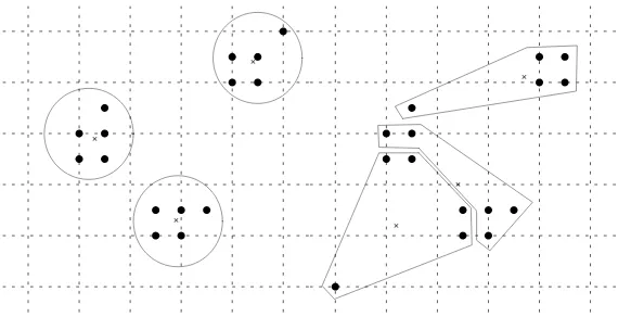
• To deal with several attributes at a time, the trivial option is to map multi-attribute data sets to univariate data by projecting the former onto a single axis (e.g., using the sum of z-scores or the first principal component, see [16]) and then use univariate microaggregation on the univariate data. Another option avoiding the information loss due to single-axis pro-jection is to usemultivariate microaggregationable to deal with unprojected multi-attribute data [21]. If we define optimal microaggregation as finding a partition in groups of size at leastksuch that within-groups homogeneity is maximum, it turns out that, while optimal univariate microaggregation can be solved in polynomial time [41], unfortunately optimal multivariate microaggregation is NP-hard [70]. is justifies the use of heuristic methods for multivariate microaggregation, such as the MDAV (Maximum Distance to Average Vector, [20, 26]). In any case, multivariate microaggregation leads to higher information loss than individual ranking [25].
To illustrate these approaches, we next give the details of the MDAV heuristic algorithm for multivariate fixed group size microaggregation on unprojected continuous data.
1. Compute the average recordxNof all records in the data set. Consider the most distant record
xr to the average recordxN (using the squared Euclidean distance).
2. Find the most distant recordxs from the recordxr considered in the previous step. 3. Form two groups around xr and xs, respectively. One group containsxr and the k 1
3.3. SYNTHETIC DATA GENERATION 21
4. If there are at least3krecords which do not belong to any of the two groups formed in Step 3, go to Step 1 taking as new data set the previous data set minus the groups formed in the last instance of Step 3.
5. If there are between3k 1and2krecords which do not belong to any of the two groups formed in Step 3: a) compute the average record xN of the remaining records; b) find the
most distant recordxr fromxN; c) form a group containingxr and thek 1records closest toxr; d) form another group containing the rest of records. Exit the algorithm.
6. If there are fewer than2krecords which do not belong to the groups formed in Step 3, form a new group with those records and exit the algorithm.
e above algorithm can be applied independently to each group of attributes resulting from partitioning the set of attributes in the data set. In [57], it has been extended to offer better utility for categorical data and in [9] to support attribute values with variable cardinality (set-valued data).
3.3 SYNTHETIC DATA GENERATION
Publication of synthetic—i.e., simulated—data was proposed long ago as a way to guard against statistical disclosure. e idea is to randomly generate data with the constraint that certain statis-tics or internal relationships of the original data set should be preserved. More than twenty years ago, Rubin suggested in [77] to create an entirely synthetic data set based on the original survey data and multiple imputation. A simulation study of this approach was given in [75].
As stated in2.5, three types of synthetic data sets are usually considered: (i) fully synthetic data sets [77], where every data item has been synthesized, (ii) partially synthetic data sets [74], where only some variables of some records are synthesized (usually the ones that present a greater risk of disclosure), and (iii) hybrid data sets [19,65], where the original data is mixed with the synthesized data.
As also stated in2.5, the generation of fully synthetic data [77] set takes three steps: (i) a model for the population is proposed, (ii) the proposed model is adjusted to the original data set, and (iii) the synthetic data set is generated by drawing from the model (without any further dependency on the original data). e utility of fully synthetic data sets is highly dependent on the accuracy of the adjusted model. If the adjusted model fits well the population, the synthetic data set should be as good as the original data set in terms of statistical analysis power. In this sense, synthetic data are superior in terms of data utility to masking techniques (which always lead to some utility loss).
to model or, even, to observe in the original data. Given that only the properties that are included in the model will be present in the synthetic data, it is important to include all the properties of the data that we want to preserve. To reduce the dependency on the models, alternatives to fully synthetic data have been proposed: partially synthetic data and hybrid data. However, using these alternative approaches to reduce the dependency on the model has a cost in terms of risk of disclosure.
As far as the risk of disclosure is concerned, the generation of fully synthetic data is consid-ered to be a very safe approach. Because the synthetic data is generated based solely on the adjusted model, analyzing the risk of disclosure of the synthetic data can be reduced to analyzing the risk of disclosure of the information about the original data that the model incorporates. Because this information is usually reduced to some statistical properties of the original data, disclosure risk is under control. In particular in fully synthetic data, they seem to circumvent the re-identification problem: since published records are invented and do not derive from any original record, it might be concluded that no individual can complain from having been re-identified. At a closer look this advantage is less clear. If, by chance, a published synthetic record matches a particular cit-izen’s non-confidential attributes (age, marital status, place of residence, etc.) and confidential attributes (salary, mortgage, etc.), re-identification using the non-confidential attributes is easy and that citizen may feel that his confidential attributes have been unduly revealed. In that case, the citizen is unlikely to be happy with or even understand the explanation that the record was synthetically generated.
Unlike fully synthetic data, neither partially synthetic nor hybrid data can circumvent re-identification. With partial synthesis, the population units in the original data set are the same population units in the partially synthetic data set. In hybrid data sets the population units in the original data set are present but mixed with synthetic ones.
On the other hand, limited data utility is another problem of synthetic data. Only the statistical properties explicitly captured by the model used by the data protector are preserved. A logical question here is why not directly publish the statistics one wants to preserve rather than release a synthetic microdata set. One possible justification for synthetic microdata would be if valid analyses could be obtained on a number of subdomains, i.e., similar results were obtained in a number of subsets of the original data set and the corresponding subsets of the synthetic data set. Partially synthetic or hybrid microdata are more likely to succeed in staying useful for subdomain analysis. e utility of the synthetic data can be improved by increasing the amount of information that the model includes about the original data. However, this is done at the cost of increasing the risk of disclosure.
See [27] for more background on synthetic data generation.
3.4 SUMMARY
3.4. SUMMARY 23
25
C H A P T E R 4
Quantifying Disclosure Risk:
Record Linkage
Record linkage (a.k.a. data matching or deduplication) was invented to improve data quality when matching files. In the context of anonymization it can be used by the data controller to empir-ically evaluate the disclosure risk associated with an anonymized data set. e data protector or controller uses a record linkage algorithm (or several such algorithms) to link each record in the anonymized data with a record in the original data set. Since the protector knows the real corre-spondence between original and protected records, he can determine the percentage of correctly linked pairs, which he uses to estimate the number of re-identifications that might be obtained by a specialized intruder. If the number of re-identifications is too high, the data set needs more anonymization by the controller before it can be released.
In its most basic approach record linkage is based on matching values of shared attributes. All the attributes that are common to both data sets are compared at once. A pair of records is said to match if the common attributes share the same values and they are the only two records sharing those values. A pair of records is said not to match if they differ in the value of some common attribute or if there are multiple pairs of records sharing those same attribute values.
Many times an attribute value may have several valid representations or variations. In that case record linkage based on exact matching of the values of common attributes is not a satisfactory approach. Rather than seeking an exact match between common attributes, a similarity function,
sim, between pairs of records is used. For a given pair of recordsxandy, the similarity function returns a value between 0 and 1 that represents the degree of similarity between the recordsxand y. It holds that:
• sim.x; y/2Œ0; 1. at is, the degree of similarity is in the range Œ0; 1with 1 meaning complete similarity and 0 meaning complete dissimilarity.
transform one string into the other; [56] proposes a measure to evaluate the semantic similarity between textual values, etc.
4.1 THRESHOLD-BASED RECORD LINKAGE
reshold-based linkage is the adaptation to similarity functions of attribute matching record linkage. Rather than saying that two records match when the values of all common attributes match, we say that they match when they are similar enough. A threshold is used to determine when two records are similar enough.
When records are to be classified between match and non-match, a single threshold value, t, is enough:
• sim.x; y/t: we classify the pair of recordsxandyas a match. • sim.x; y/ < t: we classify the pair of recordsxandyas a non-match.
e use of a sharp threshold value to distinguish between a match and a non-match may be too narrow-minded. Probably the amount of misclassifications when the similarity is near the threshold value could be large. To avoid this issue an extended classification in three classes is done: match, non-match, and potential match. e match class is used for a pair of records that have been positively identified as a match, the non-match class is used for pair of records that have been positively identified as a non-match, and the class potential match is used for a pair of records that are neither a clear match nor a clear non-match. Classification into the classes match, non-match, and potential match requires the use of two threshold valuestuandtd (with tu> td), used as follows:
• sim.x; y/tu: we classify the pair of recordsxandyas a match.
• tdsim.x; y/tu: we classify the pair of recordsxandyas a potential match. • sim.x; y/ < td: we classify the pair of recordsxandyas a non-match.
4.2 RULE-BASED RECORD LINKAGE
Basing the classification on a single value of similarity between records may sometimes be too restrictive. Imagine, for instance, that the data sets contain records related to two types of entities. It may be the case that the way to measure the similarity between records should be done in a different way for the different types of entities. is is not possible if we use a single similarity function.
4.3. PROBABILISTIC RECORD LINKAGE 27
non-match, or potential match). More formally, a classification rule is a propositional logic for-mula of the formP !C, wherePtest several similarity values combined by the logical operators
^(and),_(or), and:(not), andC is either match, non-match, or potential match. When a rule is triggered for a pair of records (the pair of records satisfy the conditions inP), the outcome of the ruleC is used to classify the pair of records.
ere are two main approaches to come up with the set of rules: generate them manually based on the domain knowledge of the data sets, or use a supervised learning approach in which pairs of records with the actual classification (match, non-match, or potential match) are passed to the system for it to automatically learn the rules.
4.3 PROBABILISTIC RECORD LINKAGE
Probabilistic record linkage [32,47] can be seen as an extension of rule-based record linkage in which the outcome of the rules is not a deterministic class in {match, non-match, potential match} but a probability distribution over the three classes. e goal in probabilistic record linkage is to come up with classification mechanisms with predetermined probabilities of misclassification (the error of classifying a pair of records related to the same entity as a non-match and the error of classifying a pair of records related to different entities as a match). Having fixed the probabilities of misclassification, we can consider the set of classification mechanisms that provide these levels of misclassification. Among these, there is one mechanism that has especially good properties and that is known as theoptimal classification mechanism. e optimal classification mechanism for some given levels of misclassification is the one that has the least probability of outputting potential match. Because pairs of records classified as potential match require further processing (by a potentially costly human expert), the optimal mechanism should be preferred over all the other classification mechanisms with given probabilities of misclassification.
Here we present a slightly simplified version of the original work in probabilistic record linkage [32]. Consider that we have two sets of entitiesX andY that are, in principle, not dis-joint. at is, a given entity can be present in bothX andY. e data sets are generated as a randomized function of the original data that accounts for the possible variations and errors of the record corresponding to an entity: forx2Xthe corresponding record is˛.x/and fory2Y the corresponding recordˇ.y/. us, even ifxDy, it may be˛.x/¤ˇ.y/and even ifx¤y, it may be˛.x/Dˇ.y/.
We use ˛.X /andˇ.Y /to represent the data sets to be linked. Linking˛.X /andˇ.Y / implies considering each pair of records of˛.X /ˇ.Y /and classifying it as either a match, a non-match, or a potential match. e set˛.X /ˇ.Y /can be split into two parts: the set of real matches
and the set of real non-matches
U D f.˛.x/; ˇ.y//Wx¤yg:
Of course,ex antedetermining the actual contents ofM andU is not possible; otherwise, there would be no need for a record linkage methodology.
Like in rule-based record linkage, the first step to determine if two records should be linked is to compute a vector of similarity functions. We define the similarity vector for˛.x/andˇ.y/ as
.˛.x/; ˇ.y//D.1.˛.x/; ˇ.y//; : : : ; k.˛.x/; ˇ.y///:
Even though we have used.˛.x/; ˇ.y//to emphasize that the vector is computed over pairs of records of˛.X /ˇ.Y /, it should be noted that the domain of isXY. e set of possible realizations of is called the comparison space and is denoted by .
For a given realization0 2 we are interested in two conditional probabilities: the
proba-bility of getting0given a real match,P .0jM /, and the probability of0given a real non-match, P .0jU /. With these probabilities we can compute theagreement ratioof0:
R.0/D P .0jM /
P .0jU /:
During the linkage we observe.˛.x/; ˇ.y//and have to decide whether.˛.x/; ˇ.y//2M (classify it as a match) or.˛.x/; ˇ.y//2U (classify it as a non-match). To account for the cases in which the decision between match and non-match is not clear, we also allow the classifica-tion of.˛.x/; ˇ.y//as a potential match. A linkage rule is used for the classification of the pair .˛.x/; ˇ.y//based on the similarity vector. us, a linkage rule is a mapping between (the comparison space) to a probability distribution over the possible classifications: match (L), non-match (N), and potential match (C).
LW ! f.pL; pN; pC/2Œ0; 13 WpLCpNCpC D1g:
Of course, a linkage rule need not always give the correct classification. A false match is a linked pair that is not a real match. A false non-match is a non-linked pair that is a real match. us, a rule can be tagged with the probability of false matches,DPL.LjU /, and with the probability of false non-matches,DPL.NjM /.
4.4. SUMMARY 29
computed and the classification is given by the rule:
8 ˆ <
ˆ :
R..˛.x/; ˇ.y///T !match
R..˛.x/; ˇ.y///T !non match
T< R..˛.x/; ˇ.y/// < T !potential
whereTandTare upper and lower threshold values. e error rates for this rule are:
D X
2 WR. /T
P .jU /:
D X
2 WR. /T
P .jM /: