Stephen Lynch
Stephen Lynch
Department of Computing and Mathematics, Manchester Metropolitan University School of Computing, Mathematics & Digital Technology, Manchester, UK
ISBN 978-3-319-06819-0 e-ISBN 978-3-319-06820-6 DOI 10.1007/978-3-319-06820-6
Springer Cham Heidelberg New York Dordrecht London Library of Congress Control Number: 2014941703
Mathematics Subject Classification (2010): 37-01, 49K15, 78A60, 28A80, 80A30, 34H10, 34K18, 70K05, 34C07, 34D06, 92B20, 94C05
© Springer International Publishing Switzerland 2014
This work is subject to copyright. All rights are reserved by the Publisher, whether the whole or part of the material is concerned, specifically the rights of translation, reprinting, reuse of illustrations, recitation, broadcasting, reproduction on microfilms or in any other physical way, and transmission or information storage and retrieval, electronic adaptation, computer software, or by similar or
dissimilar methodology now known or hereafter developed. Exempted from this legal reservation are brief excerpts in connection with reviews or scholarly analysis or material supplied specifically for the purpose of being entered and executed on a computer system, for exclusive use by the purchaser of the work. Duplication of this publication or parts thereof is permitted only under the provisions of the Copyright Law of the Publisher’s location, in its current version, and permission for use must always be obtained from Springer. Permissions for use may be obtained through RightsLink at the Copyright Clearance Center. Violations are liable to prosecution under the respective Copyright Law.
The use of general descriptive names, registered names, trademarks, service marks, etc. in this publication does not imply, even in the absence of a specific statement, that such names are exempt from the relevant protective laws and regulations and therefore free for general use.
While the advice and information in this book are believed to be true and accurate at the date of publication, neither the authors nor the editors nor the publisher can accept any legal responsibility for any errors or omissions that may be made. The publisher makes no warranty, express or implied, with respect to the material contained herein.
Printed on acid-free paper
Preface
Since the first printing of this book in 2004, MATLAB ® ; has evolved from MATLAB version 6 to MATLAB version R2014b, where presently, the package is updated twice a year. Accordingly, the second edition has been thoroughly updated and new material has been added. In this edition, there are many more applications, examples, and exercises, all with solutions, and new sections on series solutions of ordinary differential equations, perturbation methods, normal forms, Gröbner bases, and chaos synchronization have been added. There are also new chapters on image processing and binary oscillator computing.
This book provides an introduction to the theory of dynamical systems with the aid of MATLAB, the Symbolic Math Toolbox TM , the Image Processing Toolbox TM , and Simulink TM . It is written for both senior undergraduates and graduate students. Chapter 1 provides a tutorial introduction to MATLAB—new users should go through this chapter carefully whilst those moderately familiar and experienced users will find this chapter a useful source of reference. Chapters 2 – 7 deals with discrete systems, Chaps. 8 – 17 are devoted to the study of continuous systems using ordinary
differential equations and Chaps. 18 – 21 deal with both continuous and discrete systems. Chapter 22
lists three MATLAB-based examinations to be sat in a computer laboratory with access to MATLAB and Chap. 23 lists answers to all of the exercises given in the book. It should be pointed out that dynamical systems theory is not limited to these topics but also encompasses partial differential equations, integral and integro-differential equations, stochastic systems, and time-delay systems, for instance. References [1–5] given at the end of the Preface provide more information for the interested reader. The author has gone for breadth of coverage rather than fine detail and theorems with proofs are kept at a minimum. The material is not clouded by functional analytic and group theoretical definitions and so is intelligible to readers with a general mathematical background. Some of the topics covered are scarcely covered elsewhere. Most of the material in Chaps. 7, 10, 11, 15–19, and 21 is at postgraduate level and has been influenced by the author’s own research interests. There is more theory in these chapters than in the rest of the book since it is not easily accessed anywhere else. It has been found that these chapters are especially useful as reference material for senior
undergraduate project work. The theory in other chapters of the book is dealt with more comprehensively in other texts, some of which may be found in the references section of the
corresponding chapter. The book has a very hands-on approach and takes the reader from the basic theory right through to recently published research material.
MATLAB is extremely popular with a wide range of researchers from all sorts of disciplines, it has a very user-friendly interface and has extensive visualization and numerical computation
capabilities. It is an ideal package to adopt for the study of nonlinear dynamical systems; the
numerical algorithms work very quickly, and complex pictures can be plotted within seconds. The Simulink accessory to MATLAB is used for simulating dynamical processes. It is as close as one can get to building apparatus and investigating the output for a given input without the need for an actual physical model. For this reason, Simulink is very popular in the field of engineering. Note that the latest student version of MATLAB comes with a generous additional ten toolboxes including the Symbolic Math Toolbox, the Image Processing Toolbox, and Simulink.
well with one staff member to about twenty students in a computer laboratory. In most cases, I have chosen to list the MATLAB program files at the end of each chapter, this avoids unnecessary
cluttering in the text. The MATLAB programs have been kept as simple as possible and should run under later versions of the package. The MATLAB program files and Simulink model files (including updates) can even be downloaded from the Web at http://www.mathworks.com/matlabcentral/
fileexchange/authors/6536 . Readers will find that they can reproduce the figures given in the text, and then it is not too difficult to change parameters or equations to investigate other systems. Readers may be interested to hear that the MATLAB and Simulink model files have been downloaded over 30,000 times since they were uploaded in 2002 and that these files were selected as the MATLAB Central Pick of the Week in July 2013.
Chapters 2 – 7 deal with discrete dynamical systems. Chapter 2 starts with a general introduction to iteration and linear recurrence (or difference) equations. The bulk of the chapter is concerned with the Leslie model used to investigate the population of a single species split into different age classes. Harvesting and culling policies are then investigated and optimal solutions are sought. Nonlinear discrete dynamical systems are dealt with in Chap. 3 . Bifurcation diagrams, chaos, intermittency, Lyapunov exponents, periodicity, quasiperiodicity, and universality are some of the topics
introduced. The theory is then applied to real-world problems from a broad range of disciplines including population dynamics, biology, economics, nonlinear optics, and neural networks. Chapter 4
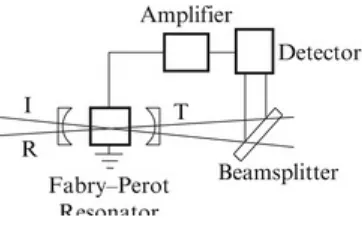
is concerned with complex iterative maps; Julia sets and the now-famous Mandelbrot set are plotted. Basins of attraction are investigated for these complex systems. As a simple introduction to optics, electromagnetic waves and Maxwell’s equations are studied at the beginning of Chap. 5 . Complex iterative equations are used to model the propagation of light waves through nonlinear optical fibers. A brief history of nonlinear bistable optical resonators is discussed and the simple fiber ring
resonator is analyzed in particular. Chapter 5 is devoted to the study of these optical resonators and phenomena such as bistability, chaotic attractors, feedback, hysteresis, instability, linear stability analysis, multistability, nonlinearity, and steady states are discussed. The first and second iterative methods are defined in this chapter. Some simple fractals may be constructed using pencil and paper in Chap. 6 , and the concept of fractal dimension is introduced. Fractals may be thought of as
identical motifs repeated on ever-reduced scales. Unfortunately, most of the fractals appearing in nature are not homogeneous but are more heterogeneous, hence the need for the multifractal theory given later in the chapter. It has been found that the distribution of stars and galaxies in our universe is multifractal, and there is even evidence of multifractals in rainfall, stock markets, and heartbeat
rhythms. Applications in materials science, geoscience, and image processing are briefly discussed. Chapter 7 provides a brief introduction to the Image Processing Toolbox TM which is being used more and more by a diverse range of scientific disciplines, especially medical imaging. The fast Fourier transform is introduced and has a wide range of applications throughout the realms of science.
Chap. 9 . Applications are taken from chemical kinetics, economics, electronics, epidemiology, mechanics, and population dynamics. The modeling of the populations of interacting species is discussed in some detail in Chap. 10 and domains of stability are discussed for the first time. Limit cycles, or isolated periodic solutions, are introduced in Chap. 11 . Since we live in a periodic world, these are the most common type of solution found when modeling nonlinear dynamical systems. They appear extensively when modeling both the technological and natural sciences.
Hamiltonian, or conservative, systems and stability are discussed in Chaps. 12, and 13 is concerned with how planar systems vary depending upon a parameter. Bifurcation, bistability, multistability, and normal forms are discussed.
The reader is first introduced to the concept of chaos in continuous systems in Chaps. 14 and 15 , where three-dimensional systems and Poincaré maps are investigated. These higher-dimensional systems can exhibit strange attractors and chaotic dynamics. One can rotate the three-dimensional objects in MATLAB and plot time series plots to get a better understanding of the dynamics involved. Once again, the theory can be applied to chemical kinetics (including stiff systems), electric circuits, and epidemiology; a simplified model for the weather is also briefly discussed. Chapter 15 deals with Poincaré first return maps that can be used to untangle complicated interlacing trajectories in higher-dimensional spaces. A periodically driven nonlinear pendulum is also investigated by means of a nonautonomous differential equation. Both local and global bifurcations are investigated in Chap. 16 . The main results and statement of the famous second part of David Hilbert’s sixteenth problem are listed in Chap. 17 . In order to understand these results, Poincaré compactification is introduced. The study of continuous systems ends with one of the author’s specialities—limit cycles of Liénard systems. There is some detail on Liénard systems, in particular, in this part of the book, but they do have a ubiquity for systems in the plane.
A brief introduction to the enticing field of neural networks is presented in Chap. 18 . Imagine trying to make a computer mimic the human brain. One could ask the question: In the future will it be possible for computers to think and even be conscious? The human brain will always be more
powerful than traditional, sequential, logic-based digital computers and scientists are trying to incorporate some features of the brain into modern computing. Neural networks perform through learning and no underlying equations are required. Mathematicians and computer scientists are attempting to mimic the way neurons work together via synapses; indeed, a neural network can be thought of as a crude multidimensional model of the human brain. The expectations are high for future applications in a broad range of disciplines. Neural networks are already being used in machine learning and pattern recognition (computer vision, credit card fraud, prediction and forecasting, disease recognition, facial and speech recognition), the consumer home entertainment market, psychological profiling, predicting wave over-topping events, and control problems, for example. They also provide a parallel architecture allowing for very fast computational and response times. In recent years, the disciplines of neural networks and nonlinear dynamics have increasingly coalesced and a new branch of science called neurodynamics is emerging. Lyapunov functions can be used to determine the stability of certain types of neural network. There is also evidence of chaos, feedback, nonlinearity, periodicity, and chaos synchronization in the brain.
Chapter 19 is devoted to the new and exciting theory behind chaos control and synchronization. For most systems, the maxim used by engineers in the past has been “stability good, chaos bad,” but more and more nowadays this is being replaced with “stability good, chaos better.” There are
Chapter 20 focuses on binary oscillator computing, the subject of UK, International and Taiwanese patents. The author and his coinventor, Jon Borresen, came up with the idea when
modeling connected biological neurons. Binary oscillator technology can be applied to the design of arithmetic logic units (ALUs), memory, and other basic computing components. It has the potential to provide revolutionary computational speedup, energy saving, and novel applications and may be applicable to a variety of technological paradigms including biological neurons, complementary metal–oxide–semiconductor (CMOS), memristors, optical oscillators, and superconducting materials. The research has the potential for MMU and industrial partners to develop super fast, low-power computers and may provide an assay for neuronal degradation for brain malfunctions such as Alzheimer’s, epilepsy, and Parkinson’s disease!
Examples of Simulink models, referred to in earlier chapters of the book, are presented in Chap.
21 . It is possible to change the type of input into the system, or parameter values, and investigate the output very quickly. This is as close as one can get to experimentation without the need for expensive equipment.
Three examination-type papers are listed in Chap. 22 and a complete set of solutions is listed in Chap. 23 .
Both textbooks and research papers are presented in the list of references. The textbooks can be used to gain more background material, and the research papers have been given to encourage further reading and independent study.
This book is informed by the research interests of the author which are currently nonlinear
ordinary differential equations, nonlinear optics, multifractals, neural networks, and binary oscillator computing. Some references include recently published research articles by the author along with an international patent.
The prerequisites for studying dynamical systems using this book are undergraduate courses in linear algebra, real and complex analysis, calculus, and ordinary differential equations; a knowledge of a computer language such as C or Fortran would be beneficial but not essential.
Recommended Textbooks
1. M.P. Coleman, An Introduction to Partial Differential Equations with MATLAB , 2nd edn.
Chapman and Hall/CRC Applied Mathematics and Nonlinear Science (Chapman and Hall/CRC, New York, 2013)
2. B. Bhattacharya, M. Majumdar, Random Dynamical Systems: Theory and Applications (Cambridge University Press, Cambridge, 2007)
3. R. Sipahi, T. Vyhlídal, S. Niculescu, P. Pepe (eds.), Time Delay Systems: Methods,
Applications and New Trends . Lecture Notes in Control and Information Sciences (Springer, New York, 2012)
4. V. Volterra, Theory of Functionals and of Integral and Integro-Differential Equations (Dover Publications, New York, 2005)
5. J. Mallet-Paret, J. Wu, H. Zhu, Y. Yi, Infinite Dimensional Dynamical Systems (Fields Institute Communications) (Springer, New York, 2013)
toolboxes come with apps. More details can be found on the relevant MathWorks web pages.
I would like to express my sincere thanks to MathWorks for supplying me with the latest versions of MATLAB and its toolboxes. Thanks also go to all of the reviewers from the editions of the Maple and Mathematica books. Special thanks go to Birkhäuser and Springer publishers. Finally, thanks to my family, especially my wife, Gaynor, and our children, Sebastian and Thalia, for their continuing love, inspiration, and support.
Contents
1 A Tutorial Introduction to MATLAB
1.1 Tutorial One: The Basics and the Symbolic Math Toolbox (1 h)
1.2 Tutorial Two: Plots and Differential Equations (1 h)
1.3 MATLAB Program Files or M-Files
1.4 Hints for Programming
1.5 MATLAB Exercises
References
2 Linear Discrete Dynamical Systems
2.1 Recurrence Relations
2.2 The Leslie Model
2.3 Harvesting and Culling Policies
2.4 MATLAB Commands
2.5 Exercises
References
3 Nonlinear Discrete Dynamical Systems
3.1 The Tent Map and Graphical Iterations
3.2 Fixed Points and Periodic Orbits
3.3 The Logistic Map, Bifurcation Diagram, and Feigenbaum Number
3.4 Gaussian and Hénon Maps
3.5 Applications
3.6 MATLAB Program Files
References
4 Complex Iterative Maps
4.1 Julia Sets and the Mandelbrot Set
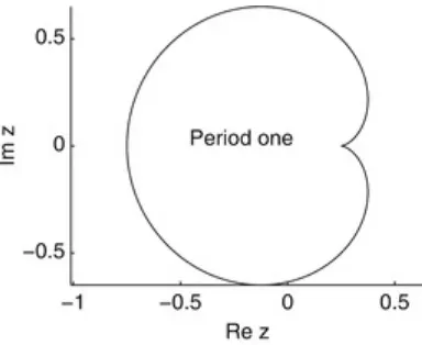
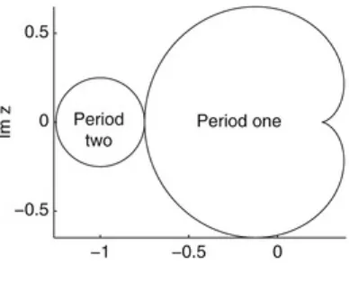
4.2 Boundaries of Periodic Orbits
4.3 MATLAB Commands
4.4 Exercises
References
5 Electromagnetic Waves and Optical Resonators
5.1 Maxwell’s Equations and Electromagnetic Waves
5.2 Historical Background
5.3 The Nonlinear SFR Resonator
5.4 Chaotic Attractors and Bistability
5.5 Linear Stability Analysis
5.6 Instabilities and Bistability
5.7 MATLAB Commands
5.8 Exercises
References
6 Fractals and Multifractals
6.1 Construction of Simple Examples
6.2 Calculating Fractal Dimensions
6.3 A Multifractal Formalism
6.4 Multifractals in the Real World and Some Simple Examples
6.5 MATLAB Commands
References
7 The Image Processing Toolbox
7.1 Image Processing and Matrices
7.2 The Fast Fourier Transform
7.3 The Fast Fourier Transform on Images
7.4 Exercises
References
8 Differential Equations
8.1 Simple Differential Equations and Applications
8.2 Applications to Chemical Kinetics
8.3 Applications to Electric Circuits
8.4 Existence and Uniqueness Theorem
8.5 MATLAB Commands
8.6 Exercises
References
9 Planar Systems
9.1 Canonical Forms
9.2 Eigenvectors Defining Stable and Unstable Manifolds
9.3 Phase Portraits of Linear Systems in the Plane
9.4 Linearization and Hartman’s Theorem
9.5 Constructing Phase Plane Diagrams
9.6 MATLAB Commands
9.7 Exercises
10 Interacting Species
10.1 Competing Species
10.2 Predator-Prey Models
10.3 Other Characteristics Affecting Interacting Species
10.4 MATLAB Commands
10.5 Exercises
References
11 Limit Cycles
11.1 Historical Background
11.2 Existence and Uniqueness of Limit Cycles in the Plane
11.3 Nonexistence of Limit Cycles in the Plane
11.4 Perturbation Methods
11.5 MATLAB Commands
11.6 Exercises
References
12 Hamiltonian Systems, Lyapunov Functions, and Stability
12.1 Hamiltonian Systems in the Plane
12.2 Lyapunov Functions and Stability
12.3 MATLAB Commands
12.4 Exercises
References
13 Bifurcation Theory
13.1 Bifurcations of Nonlinear Systems in the Plane
13.3 Multistability and Bistability
13.4 MATLAB Commands
13.5 Exercises
References
14 Three-Dimensional Autonomous Systems and Chaos
14.1 Linear Systems and Canonical Forms
14.2 Nonlinear Systems and Stability
14.3 The Rössler System and Chaos
14.4 The Lorenz Equations, Chua’s Circuit, and the Belousov–Zhabotinski Reaction
14.5 MATLAB Commands
14.6 Exercises
References
15 Poincaré Maps and Nonautonomous Systems in the Plane
15.1 Poincaré Maps
15.2 Hamiltonian Systems with Two Degrees of Freedom
15.3 Nonautonomous Systems in the Plane
15.4 MATLAB Commands
15.5 Exercises
References
16 Local and Global Bifurcations
16.1 Small-Amplitude Limit Cycle Bifurcations
16.2 Gröbner Bases
16.3 Melnikov Integrals and Bifurcating Limit Cycles from a Center
16.5 MATLAB and MuPAD Commands
16.6 Exercises
References
17 The Second Part of Hilbert’s Sixteenth Problem
17.1 Statement of Problem and Main Results
17.2 Poincaré Compactification
17.3 Global Results for Liénard Systems
17.4 Local Results for Liénard Systems
17.5 Exercises
References
18 Neural Networks
18.1 Introduction
18.2 The Delta Learning Rule and Backpropagation
18.3 The Hopfield Network and Lyapunov Stability
18.4 Neurodynamics
18.5 MATLAB Commands
18.6 Exercises
References
19 Chaos Control and Synchronization
19.1 Historical Background
19.2 Controlling Chaos in the Logistic Map
19.3 Controlling Chaos in the Hénon Map
19.4 Chaos Synchronization
19.6 Exercises
References
20 Binary Oscillator Computing
20.1 Brain-Inspired Computing
20.2 Oscillatory Threshold Logic
20.3 Applications and Future Work
20.4 MATLAB Commands
20.5 Exercises
References
21 Simulink
21.1 Introduction
21.2 Electric Circuits
21.3 A Mechanical System
21.4 Nonlinear Optics
21.5 The Lorenz Equations and Chaos Synchronization
21.6 Exercises
References
22 Examination-Type Questions
22.1 Examination 1
22.2 Examination 2
22.3 Examination 3
23 Solutions to Exercises
23.1 Chapter 1
23.3 Chapter 3
23.4 Chapter 4
23.5 Chapter 5
23.6 Chapter 6
23.7 Chapter 7
23.8 Chapter 8
23.9 Chapter 9
23.10 Chapter 10
23.11 Chapter 11
23.12 Chapter 12
23.13 Chapter 13
23.14 Chapter 14
23.15 Chapter 15
23.16 Chapter 16
23.17 Chapter 17
23.18 Chapter 18
23.19 Chapter 19
23.20 Chapter 20
23.21 Chapter 21
23.22 Chapter 22
(1)
© Springer International Publishing Switzerland 2014
Stephen Lynch, Dynamical Systems with Applications using MATLAB®, DOI 10.1007/978-3-319-06820-6_1
1. A Tutorial Introduction to MATLAB
Stephen Lynch
1Department of Computing and Mathematics, Manchester Metropolitan University School of Computing, Mathematics & Digital Technology, Manchester, UK
Aims and Objectives
To provide a tutorial guide to MATLAB
To give practical experience in using the package To promote self-help using the online help facilities
To provide a concise source of reference for experienced users On completion of this chapter the reader should be able to
use MATLAB and the Symbolic Math Toolbox; produce simple MATLAB programs;
access some MATLAB commands and programs over the World Wide Web.
It is assumed that the reader is familiar with either the Windows or UNIX platform. This book was prepared using MATLAB R2014b, but most programs should work under earlier and later versions of the package.
The commands and programs listed have been chosen to allow the reader to become familiar with MATLAB and the Symbolic Math Toolbox within a few hours. They provide a concise summary of the type of commands that will be used throughout this book. New users should be able to start on their own problems after completing this tutorial, and experienced users should find this chapter an excellent source of reference. Of course, there are many MATLAB textbooks on the market for those who require further applications or more detail. Note that from version 5, the Symbolic Math
Toolbox is powered by the MuPAD symbolic engine, and nearly all Symbolic Math Toolbox
functions work the same way as in previous versions. The Symbolic Math Toolbox provides tools for solving and manipulating symbolic math expressions and performing variable-precision arithmetic. The toolbox contains hundreds of MATLAB symbolic functions that leverage the MuPAD engine for tasks such as differentiation, integration, simplification, transforms, and equation solving. See the online MATLAB Help pages if you require further information.
If you experience any problems, there are several options for you to take. There is an excellent index within MATLAB, there are thousands of textbooks, see references [1–10], for example, and MATLAB program files (or M-files) can be downloaded from the MATLAB Central File Exchange at the link
Download the zipped M-files and extract the relevant M-files from the archive onto your computer. Since 2002, the author’s files associated with the first edition of this book have been downloaded over 30,000 times by users from all over the world.
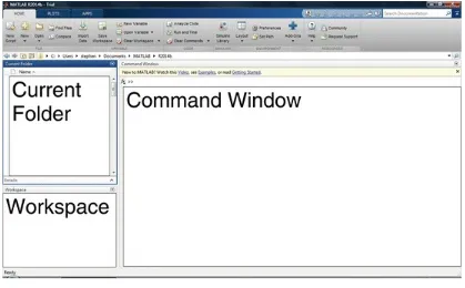
To start MATLAB, simply double-click on the MATLAB icon. In the UNIX environment, one types MATLAB as a shell command. The author has used the Windows platform in the preparation of this material. When MATLAB starts up, by default three windows are displayed entitled Current Folder, Command Window, and Workspace. Figure 1.1 shows a typical screen when running MATLAB. Each of the windows appearing in Fig. 1.1 will now be described:
Fig. 1.1 The MATLAB user interface
Current Folder. This window shows the current folder where files are listed. Note that when typing in the Command Window, the command pwd also displays the MATLAB current folder.
Command Window. This is where the user types in MATLAB commands followed by the RETURN or ENTER key on the keyboard. If you do not want to see the result (e.g., you would not want to see a list of numbers from 1 to 1,000), then use the semicolon delimiter.
Workspace. The workspace consists of the set of variables built up during a session of using the MATLAB software and stored in memory.
The Command Window is where the MATLAB commands are typed and executed, and this is where the user can use MATLAB just like a graphing calculator. When in the Command Window, command lines may be returned to and edited using the up and down arrow keys. If you do make a typing error, MATLAB will give an error: message and even point to the mistake in the code. Do not re-type the line, simply use the up arrow key and edit your mistake. To clear the Command Window simply type >> clc after the command prompt.
1.
2.
3.
4.
5.
6.
1.
2.
3.
results obtained with MATLAB should be verified by experiment where possible. Some Well-Known Pitfalls of MATLAB
Array indices start with 1 and not 0. In some programs a translation may be required to start indices with zero.
MATLAB allows use of variable names of pre-defined functions. For example, you can set rand = 1 which means that you cannot subsequently use the rand command. Readers should use the which command to check variable names.
Take care with element-wise and matrix-matrix multiplication.
Some functions such as max, min, sort, sum, mean, etc., behave differently for complex and real data.
In MATLAB it is better (though not easier) to use matrix or vector operations instead of loops in programs.
Without the Symbolic Math Toolbox, MATLAB gives approximate answers.
The reader should also be aware that even when the programs run successfully the output may not be correct. The following phenomena can greatly affect the results obtained for nonlinear dynamical systems:
Chaos and sensitivity to initial conditions.
Using the correct numerical solver for your particular problem.
1.1 Tutorial One: The Basics and the Symbolic Math Toolbox (1 h)
There is no need to copy the comments, they are there to help you. Click on the MATLAB icon and copy the command after the >> prompt. Press Return at the end of a line to see the answer or use asemicolon to suppress the output. You can interrupt a computation at any time by holding Ctrl+C. This tutorial should be run in the Command Window .
MATLAB commands Comments
>> % This is a comment. % Helps when writing
% programs.
>> 3^2*4-3*2^5*(4-2) % Simple arithmetic.
>> sqrt(16) % The square root.
>> % Vectors and Matrices.
>> u=1:2:9 % A vector u=(1,3,5,7,9).
>> v=u.^2 % A vector v=(1,9,25,49,81).
>> A=[1,2;3,4] % A is a 2 by 2 matrix.
>> A’ % The transpose of matrix A.
>> det(A) % The determinant of a matrix.
>> B=[0,3,1;0.3,0,0;0,0.5,0] % B is a 3 by 3 matrix.
>> eig(B) % The eigenvalues of B.
>> % List the eigenvectors and eigenvalues of B. >> [Vects,Vals]=eig(B)
>> C=[100;200;300] % A 3 by 1 matrix.
>> D=B*C % Matrix multiplication.
>> E=B^4 % Powers of a matrix.
>> % Complex numbers.
>> % The semicolons suppress the output. >> z1=1+i;z2=1-i;z3=2+i;
>> z4=2*z1-z2*z3 % Simple arithmetic.
>> abs(z1) % The modulus.
>> real(z1) % The real part.
>> imag(z1) % The imaginary part.
>> exp(i*z1) % Returns a complex number.
>> % The Symbolic Math Toolbox.
>> sym(1/2)+sym(3/4) % Symbolic evaluation.
>> % Double precision floating point arithmetic. >> 1/2+3/4
>> % Variable precision arithmetic (50 sig figs). >> vpa(pi,50)
>> syms x y z % Symbolic objects.
>> z=x^3-y^3
>> factor(z) % Factorization.
>> % Symbolic expansion of the last answer. >> expand(ans)
>> simplify(z/(x-y)) % Symbolic simplification.
>> % Symbolic solution of algebraic equations. >> [x,y]=solve(’x^2-x’,’2*x*y-y^2’)
>> syms x mu
>> f=mu*x*(1-x) % Define a function.
>> fof=subs(f,x,f) % A function of a function.
>> limit(x/sin(x),x,0) % Limits.
>> diff(f,x) % Differentiation.
>> % Partial differentiation, (with respect to y twice). >> syms x y
>> diff(x^2+3*x*y-2*y^2,y,2)
>> int(sin(x)*cos(x),x,0,pi/2) % Integration.
>> int(1/x,x,0,inf) % Improper integration.
>> syms n s w x
>> s1=symsum(1/n^2,1,inf) % Symbolic summation.
>> g=exp(x)
>> taylor(g,’Order’,10) % Taylor series expansion.
>> syms x s
>> laplace(x^3) % Laplace transform.
>> ilaplace(6/s^4) % Inverse Laplace transform.
>> syms x w
>> fourier(-2*pi*abs(x)) % Fourier transform.
>> ifourier(4*pi/w^2) % Inverse Fourier transform.
>> quit % Exit MATLAB.
>> % End of Tutorial 1.
1.2 Tutorial Two: Plots and Differential Equations (1 h)
More involved plots will be dealt with in Sect. 1.3. You will need the Symbolic Math Toolbox for most of the commands in this section.
MATLAB Commands
>> % Plotting graphs.>> % Set up the domain and plot a simple function. >> x=-2:.01:2;
>> plot(x,x.^2)
>> % Plot two curves on one graph and label them. >> t=0:.1:100;
>> y1=exp(-.1.*t).*cos(t);y2=cos(t); >> plot(t,y1,t,y2),legend(’y1’,’y2’)
>> % Plotting with the Symbolic Math Toolbox. >> ezplot(’x^2’,[-2,2])
>> % Plot with labels and title.
>> ezplot(’exp(-t)*sin(t)’),xlabel(’time’),ylabel(’current’), title(’decay’)
>> % Contour plot on a grid of 50 by 50. >> ezcontour(’y^2/2-x^2/2+x^4/4’,[-2,2],50)
>> % Surface plot. Rotate the plot using the mouse. >> ezsurf(’y^2/2-x^2/2+x^4/4’,[-2,2],50)
>> ezplot(’t^3-4*t’,’t^2’,[-3,3]) >> % 3-D parametric curve.
>> ezplot3(’sin(t)’,’cos(t)’,’t’,[-10,10]) >> % Implicit plot.
>> ezplot(’2*x^2+3*y^2-12’)
Symbolic Solutions to Ordinary Differential Equations (ODEs). If an analytic solution cannot be found, the message “Warning: Explicit solution could not be found” is shown.
>> % The D denotes differentiation with respect to t. >> dsolve(’Dx=-x/t’)
>> % An initial value problem. >> dsolve(’Dx=-t/x’,’x(0)=1’) >> % A second order ODE.
>> dsolve(’D2x+5*Dx+6*x=10*sin(t)’,’x(0)=0’,’Dx(0)=0’) >> % A linear system of ODEs.
>> [x,y]=dsolve(’Dx=3*x+4*y’,’Dy=-4*x+3*y’) >> % A system with initial conditions.
>> [x,y]=dsolve(’Dx=x^2’,’Dy=y^2’,’x(0)=1,y(0)=1’) >> % A 3-D linear system.
>> [x,y,z]=dsolve(’Dx=x’,’Dy=y’,’Dz=-z’)
Numerical Solutions to ODEs. These methods are usually used when an analytic solution cannot be found—even though one may exist! Below is a Table 1.1 lists some initial value problem solvers in MATLAB. See the on-line MATLAB index for more details or type >> help topic.
Table 1.1 There are other solvers, but the solvers listed below should suffice for the material covered in this book
Solver O.D.E Method Summary
ode45 Nonstiff Runge–Kutta Try this first ode23 Nonstiff Runge–Kutta Crude tolerances ode113 Nonstiff Adams Multi-step solver ode15s Stiff Gears method If you suspect stiffness ode23s Stiff Rosenbrock One step solver
>> % Set up a 1-D system with initial condition 50, >> % and run for 0<t<100.
>> deq1=@(t,x) x(1)*(.1-.01*x(1)); >> [t,xa]=ode45(deq1,[0 100],50); >> plot(t,xa(:,1))
>> % A 2-D system with initial conditions [.01,0], >> % and run for 0<t<50.
>> deq2=@(t,x) [.1*x(1)+x(2);-x(1)+.1*x(2)]; >> [t,xb]=ode45(deq2,[0 50],[.01,0]);
>> plot(xb(:,1),xb(:,2))
>> % A 3-D system with initial conditions.
>> deq3=@(t,x) [x(3)-x(1);-x(2);x(3)-17*x(1)+16]; >> [t,xc]=ode45(deq3,[0 20],[.8,.8,.8]);
>> plot3(xc(:,1),xc(:,2),xc(:,3))
>> deq4=@(t,x) [x(2);1000*(1-(x(1))^2)*x(2)-x(1)]; >> [t,xd]=ode23s(deq4,[0 3000],[.01,0]);
>> plot(xd(:,1),xd(:,2))
>> % Displacement against time. >> plot(t,xd(:,1))
>> % End of Tutorial 2.
1.3 MATLAB Program Files or M-Files
Sections 1.1 and 1.2 illustrate the use of the Command Window and its interactive nature. More involved tasks will require more lines of code, and it is better to use MATLAB program files or M-files. Each program is displayed between horizontal lines and kept short to aid in understanding; the output is also included.
Function M-Files. The following M-file defines the logistic function. % Program 1 - The logistic function.
% Save the M-file as fmu.m. function y=fmu(mu,x)
y=mu*x*(1-x);
% End of Program 1. >> fmu(2,.1)
ans = 0.1800
The for..end Loop. For repetitive tasks.
% Program 2 - The Fibonacci sequence. % Save the M-file as Fibonacci.m.
Nmax=input(’Input the number of terms of the Fibonacci sequence:’)
Input the number of terms of the Fibonacci sequence:10 Nmax=10
F = 1 1 2 3 5 8 13 21 34 55
Conditional Statements. If..then..elseif..else..end, etc.
% Program 3 - The use of logical expressions. % Save this M-file as test1.m.
integer=input(’Which integer do you wish to test?’) if integer == 0
disp([’The integer is zero.’]) elseif integer < 0
disp([’The integer is positive.’]) end
% End of Program 3. >> test1
Which integer do you wish to test?-100 integer=-100
The integer is negative.
Fig. 1.2 A multiple plot with text
Graphic Programs. Multiple plots with text (Fig. 1.2).
% Program 4 - Two curves on one graph. % Save the M-file as plot1.m.
% Tex symbols can be plotted within a figure window. clear all
title(’Two curves on one plot’,’Fontsize’,fsize) % End of Program 4.
>> plot1
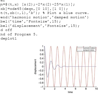
Labeling Solution Curves. Solutions to the pendulum problem (Fig. 1.3). % Program 5 - Solution curves to different ODEs. % Save M-file as deplot1.m.
clear; figure; hold on
deqn=@(t,x) [x(2);-25*x(1)];
plot(t,xa(:,1),’r’); % Plot a red curve. clear
deqn=@(t,x) [x(2);-2*x(2)-25*x(1)]; [t,xb]=ode45(deqn,[0 10],[1 0]);
plot(t,xb(:,1),’b’); % Plot a blue curve. legend(’harmonic motion’,’damped motion’)
Fig. 1.3 Harmonic and damped motion of a pendulum
Echo Commands. Useful when debugging a program.
% Program 6 - Use echo to display command lines. % Save the M-file as poincare.m.
echo on
r = 1.0000 0.1373 0.0737 0.0504 0.0383
1.4 Hints for Programming
The MATLAB language contains very powerful commands, which means that some complex
(a)
(b) 1.
following does not help you with your particular problem.
Common Typing Errors. The author strongly advises new users to run Tutorials One and Two in the Command Window environment, this should reduce typing errors.
Be careful to include all mathematics operators.
When dealing with vectors put a full stop (.) in front of the mathematical operator. Make sure brackets, parentheses, etc. match up in correct pairs.
Remember MATLAB is case-sensitive.
Check the syntax, enter help followed by the name of the command.
Programming Tips. The reader should use the M-files in Sect. 1.3 to practice simple
programming techniques. Note that MATLAB has a built in code analyzer and appears in the top right corner of the message bar. Red indicates syntax errors were detected. Orange indicates warnings or opportunities for improvement, but no errors, were detected, and green indicates no errors, warnings, or opportunities for improvement were detected. For more information and examples, the reader should check the MathWorks document center for checking code for errors and warnings.
It is best to clear values at the start of a large program. Use the figure command when creating a new figure.
Preallocate arrays to prevent MATLAB from having to continually re-size arrays—for example, use the zeros command. An example is given in Program 2 above.
Vectorize where possible. Convert for and while loops to equivalent vector or matrix operations.
If a program involves a large number of iterations, for example 50,000, then run it for three iterations first of all and use the echo command.
If the computer is not responding hold Ctrl+C and try reducing the size of the problem. Click on the green play Run in the M-file Window, MATLAB will list any error messages. Find a similar M-file in a book or on the Web, and edit it to meet your needs.
Make sure you have the correct packages, for example, the symbolic commands will not work if you do not have the Symbolic Math Toolbox.
Check which version of MATLAB you are using.
1.5 MATLAB Exercises
Evaluate the following:;
(c)
(d)
(e)
(a)
(b)
(c)
(d)
(e) 2.
(a) 3.
sin(0. 1π);
;
.
Given that
determine the following: A + 4BC;
the inverse of each matrix if it exists;
A3;
the determinant of C;
the eigenvalues and eigenvectors of B.
Given that , , and , evaluate the following:
(b)
(c)
(d)
(e)
(a)
(b)
(c)
(d)
(e) 4.
;
;
ln(z 1);
sin(z 3).
Evaluate the following limits if they exist:
;
;
;
;
(a)
(b)
(c)
(d)
(e) 5.
(a)
(b)
(c)
(d)
(e) 6.
Find the derivatives of the following functions:
;
;
y = e xsinxcosx;
y = tanhx;
.
Evaluate the following definite integrals:
;
;
;
;
(a)
(b)
(c)
(d)
(e) 7.
(a)
(b)
(c) 8.
Graph the following:
;
, for − 5 ≤ x ≤ 5;
;
, for − 3 ≤ x ≤ 3 and − 1 ≤ y ≤ 1;
, , for − 4 ≤ t ≤ 4.
Solve the following differential equations:
, given that y(1) = 1;
, given that y(2) = 3;
(d)
(e)
9.
10.
, given that x(0) = 1 and ;
, given that x(0) = 1 and .
Carry out one hundred iterations on the recurrence relation
given that (a) x 0 = 0. 2 and (b) x 0 = 0. 2001. List the final ten iterates in each case.
Type “help while” after the >> prompt to read information on the while command. Use a while
loop to program Euclid’s algorithm for finding the greatest common divisor of two integers. Use your program to find the greatest common divisor of 12,348 and 14,238.
References
1. S. Attaway, MATLAB: A Practical Introduction to Programming and Problem Solving, 2nd edn. (Butterworth-Heinemann, Newton, 2011)
2. O. Demirkaya, M.H. Asyali, P.K. Sahoo, Image Processing with MATLAB: Applications in Medicine and Biology (CRC Press, New York, 2008)
3. D.G. Duffy, Advanced Engineering Maths with MATLAB, 3rd edn. (CRC Press, New York, 2010)
4. A. Gilat, MATLAB: An Introduction with Applications, 5th edn. (Wiley, New York, 2014)
5. B.R. Hunt, R.L. Lipman, J.M. Rosenberg, A Guide to MATLAB: For Beginners and Experienced Users, 3rd edn. (Cambridge University Press, Cambridge, 2014)
6. H. Moore, MATLAB for Engineers, 2nd edn. (Prentice-Hall, Upper Saddle River, 2008)
7. R. Pratab, MATLAB: Getting Started with MATLAB: A Quick Introduction for Scientists and Engineers (Oxford University Press, Oxford, 2009)
8. M. Shahin, Explorations of Mathematical Models in Biology with MATLAB (Wiley-Blackwell, New York, 2014)
9. A. Siciliano, Matlab: Data Analysis and Visualization (World Scientific, Singapore, 2008)
(1)
© Springer International Publishing Switzerland 2014
Stephen Lynch, Dynamical Systems with Applications using MATLAB®, DOI 10.1007/978-3-319-06820-6_2
2. Linear Discrete Dynamical Systems
Stephen Lynch
1Department of Computing and Mathematics, Manchester Metropolitan University School of Computing, Mathematics & Digital Technology, Manchester, UK
Aims and Objectives
To introduce recurrence relations for first- and second-order difference equations To introduce the theory of the Leslie model
To apply the theory to modeling the population of a single species On completion of this chapter, the reader should be able to
solve first- and second-order homogeneous linear difference equations; find eigenvalues and eigenvectors of matrices;
model a single population with different age classes;
predict the long-term rate of growth/decline of the population; investigate how harvesting and culling policies affect the model.
This chapter deals with linear discrete dynamical systems, where time is measured by the number of iterations carried out and the dynamics are not continuous. In applications this would imply that the solutions are observed at discrete time intervals.
Recurrence relations can be used to construct mathematical models of discrete systems. They are also used extensively to solve many differential equations which do not have an analytic solution; the differential equations are represented by recurrence relations (or difference equations) that can be solved numerically on a computer. Of course one has to be careful when considering the accuracy of the numerical solutions. Ordinary differential equations are used to model continuous dynamical systems later in the book.
The bulk of this chapter is concerned with a linear discrete dynamical system that can be used to model the population of a single species. As with continuous systems, in applications to the real world, linear models generally produce good results over only a limited range of time. The Leslie model introduced here is useful when establishing harvesting and culling policies. Nonlinear discrete dynamical systems will be discussed in the next chapter.
2.1 Recurrence Relations
This section is intended to give the reader a brief introduction to difference equations and illustrate the theory with some simple models.
First-Order Difference Equations
A recurrence relation can be defined by a difference equation of the form
(2.1) where x n+1 is derived from x n and n = 0, 1, 2, 3, …. If one starts with an initial value, say, x 0, then iteration of (2.1) leads to a sequence of the form
In applications, one would like to know how this sequence can be interpreted in physical terms. Equations of the form (2.1) are called first-order difference equations because the suffices differ by one. Consider the following simple example.
Example 1.
The difference equation used to model the interest in a bank account compounded once per year is given by
Find a general solution and determine the balance in the account after 5 years given that the initial deposit is 10,000 dollars and the interest is compounded annually.
Solution.
Using the recurrence relation
and, in general,
where n = 0, 1, 2, 3, …. Given that x 0 = 10, 000 and n = 5, the balance after 5 years will be x 5 = 11, 592. 74 dollars.
Theorem 1.
The general solution of the first-order linear difference equation
Proof.
Applying the recurrence relation given in (2.2)
and the pattern in general is
Using geometric series, , provided that m ≠ 1. If m = 1, then the sum of the geometric sequence is n. This concludes the proof of Theorem 1. Note that if | m | < 1, then
as n → ∞. □
Second-Order Linear Difference Equations
Recurrence relations involving terms whose suffices differ by two are known as second-order linear difference equations . The general form of these equations with constant coefficients is
(2.3) Theorem 2.
The general solution of the second-order recurrence relation (2.3) is
where k 1 ,k 2 are constants and λ 1 ≠ λ 2 are the roots of the quadratic equation . If λ 1 = λ 2 , then the general solution is of the form
Note that when λ 1 and λ 2 are complex, the general solution can be expressed as
where A and B are constants. When the eigenvalues are complex , the solution oscillates and is real.
Proof.
The solution of system (2.2) gives us a clue where to start. Assume that x n = λ n k is a solution,
where λ and k are to be found. Substituting, (2.3) becomes
or
(i)
(ii)
(iii)
(i)
(2.4) Equation (2.4) is called the characteristic equation . The difference equation (2.3) has two solutions, and because the equation is linear, a solution is given by
where λ 1 ≠ λ 2 are the roots of the characteristic equation. If λ 1 = λ 2, then the characteristic equation can be written as
Therefore, b = 2a λ 1 and . Now assume that another solution is of the form kn λ n .
Substituting, (2.3) becomes
therefore
which equates to zero from the above. This confirms that kn λ n is a solution to (2.3). Since the system is linear, the general solution is thus of the form
□
The values of k jcan be determined if x 0 and x 1 are given. Consider the following simple examples.
Example 2.
Solve the following second-order linear difference equations: , given that x 0 = 1 and x 1 = 2;
, given that x 0 = 1 and x 1 = 3;
, given that x 0 = 1 and x 1 = 2.
Solution.
The characteristic equation is
which has roots at λ 1 = 3 and . The general solution is therefore
(ii)
(iii)
The characteristic equation is
which has a repeated root at λ 1 = 2. The general solution is
Substituting for x 0 and x 1, gives the solution
The characteristic equation is
which has complex roots and . The general solution is
Substituting for λ 1 and λ 2 the general solution becomes
Substituting for x 0 and x 1 gives and , and so
Example 3.
Suppose that the national income of a small country in year n is given by , where S n , P n, and G n represent national spending by the populous, private investment, and government
spending, respectively. If the national income increases from 1 year to the next, then assume that consumers will spend more the following year; in this case, suppose that consumers spend of the previous year’s income, then . An increase in consumer spending should also lead to
increased investment the following year; assume that . Substitution for S nthen gives . Finally, assume that the government spending is kept constant. Simple
manipulation then leads to the following economic model
(i)
(ii)
(iii)
(i)
(ii)
(iii)
where I nis the national income in year n and G is a constant. If the initial national income is G dollars and 1 year later is dollars, determine
a general solution to this model;
the national income after 5 years; and
the long-term state of the economy.
Solution.
The characteristic equation is given by
which has solutions and . Equation (2.5) also has a constant term G. Assume that the solution involves a constant term also; try I n = k 3 G, then from (2.5)
and so . Therefore, a general solution is of the form
Given that I 0 = G and , simple algebra gives and k 2 = 3. When n = 5, I 5 = 2. 856G, to three decimal places.
As n → ∞, I n → 3G, since | λ 1 | < 1 and | λ 2 | < 1. Therefore, the economy stabilizes in the long term to a constant value of 3G. This is obviously a very crude model.
A general n-dimensional linear discrete population model is discussed in the following sections using matrix algebra.
2.2 The Leslie Model
portion of a species. For most species the number of females is equal to the number of males, and this assumption is made here. The model can be applied to human populations, insect populations, and animal and fish populations. The model is an example of a discrete dynamical system. As explained throughout the text, we live in a nonlinear world and universe; since this model is linear, one would expect the results to be inaccurate in the long term. However, the model can give some interesting results, and it incorporates some features not discussed in later chapters. The following
characteristics are ignored—diseases, environmental effects, and seasonal effects. The book [8] provides an extension of the Leslie model, investigated in this chapter and most of the [1–7] cited here, where individuals exhibit migration characteristics. A nonlinear Leslie matrix model for predicting the dynamics of biological populations in polluted environments is discussed in [7]. Assumptions:
The females are divided into n age classes ; thus, if N is the theoretical maximum age attainable by a female of the species, then each age class will span a period of equally spaced, days, weeks,
months, years, etc. The population is observed at regular discrete time intervals which are each equal to the length of one age class. Thus, the kth time period will be given by . Define to be the number of females in the ith age class after the kth time period. Let b idenote the number of female offspring born to one female during the ith age class, and let c ibe the proportion of females which continue to survive from the ith to the (i + 1)st age class.
In order for this to be a realistic model the following conditions must be satisfied:
Obviously, some b ihave to be positive in order to ensure that some births do occur and no c iare zero; otherwise, there would be no females in the (i + 1)st age class.
Working with the female population as a whole, the following sets of linear equations can be derived. The number of females in the first age class after the kth time period is equal to the number of females born to females in all n age classes between the time t k−1 and t k ; thus,
The number of females in the (i + 1)st age class at time t k is equal to the number of females in the ith age class at time t k−1 who continue to survive to enter the (i + 1)st age class; hence,
Equations of the above form can be written in matrix form, and so
(a)
(b)
(c)
where and the matrix L is called the Leslie matrix .
Suppose that X (0) is a vector giving the initial number of females in each of the n age classes, then
Therefore, given the initial age distribution and the Leslie matrix L, it is possible to determine the female age distribution at any later time interval.
Example 4.
Consider a species of bird that can be split into three age groupings: those aged 0–1 year, those aged 1–2 years, and those aged 2–3 years. The population is observed once a year. Given that the Leslie matrix is equal to
and the initial population distribution of females is , , and , compute the number of females in each age group after
10 years;
20 years;
50 years.
Solution.
(a)
(b)
(c)
(i)
(ii)
(iii)
(iv)
The numbers are rounded down to whole numbers since it is not possible to have a fraction of a living bird. Obviously, the populations cannot keep on growing indefinitely. However, the model does give useful results for some species when the time periods are relatively short.
In order to investigate the limiting behavior of the system it is necessary to consider the
eigenvalues and eigenvectors of the matrix L. These can be used to determine the eventual population distribution with respect to the age classes.
Theorem 3.
Let the Leslie matrix L be as defined above and assume that b i ≥ 0 for 1 ≤ i ≤ n;
at least two successive b i are strictly positive; and
0 < c i ≤ 1 for 1 ≤ i < n.
Then,
matrix L has a unique positive eigenvalue, say, λ 1 ;
λ 1 is simple or has algebraic multiplicity one;
the eigenvector—X 1 , say—corresponding to λ 1 has positive components;
any other eigenvalue, λ i ≠ λ 1 , of L satisfies
and the positive eigenvalue λ 1 is called strictly dominant .
Assume that x 1 = 1, then a possible eigenvector corresponding to λ 1 is given by
Assume that L has n linearly independent eigenvectors, say, X 1, X 2, …, X n. Therefore, L is diagonizable. If the initial population distribution is given by X (0) = X
0, then there exist constants b 1, b 2, …, b n, such that
Since
then
Therefore,
Since λ 1 is dominant, for λ i≠ λ 1, and as k → ∞. Thus, for large k,
In the long run, the age distribution stabilizes and is proportional to the vector X 1. Each age group will change by a factor of λ 1 in each time period. The vector X 1 can be normalized so that its
components sum to one, the normalized vector then gives the eventual proportions of females in each of the n age groupings.
Note that if λ 1 > 1, the population eventually increases; if λ 1 = 1, the population stabilizes and if λ 1 < 1, the population eventually decreases.
Example 5.
Determine the eventual distribution of the age classes for Example 4.
Solution.
The characteristic equation is given by
to three decimal places. Note that λ 1 is the dominant eigenvalue. To find the eigenvector corresponding to λ 1, solve
One solution is , and x 3 = 0. 420. Divide each term by the sum to obtain the normalized eigenvectors
Hence, after a number of years, the population will increase by approximately 2. 3 % every year. The percentage of females aged 0–1 year will be 69. 6 %, aged 1–2 years will be 20. 4 %, and aged 2–3 years will be 10 %.
2.3 Harvesting and Culling Policies
This section will be concerned with insect and fish populations only since they tend to be very large. The model has applications when considering insect species which survive on crops, for
example. An insect population can be culled each year by applying either an insecticide or a predator species. Harvesting of fish populations is particularly important nowadays; certain policies have to be employed to avoid depletion and extinction of the fish species. Harvesting indiscriminately could cause extinction of certain species of fish from our oceans.
A harvesting or culling policy should only be used if the population is increasing.
Definition 1.
A harvesting or culling policy is said to be sustainable if the number of fish, or insects, killed and the age distribution of the population remaining are the same after each time period.
Assume that the fish or insects are killed in short sharp bursts at the end of each time period. Let X be the population distribution vector for the species just before the harvesting or culling is applied. Suppose that a fraction of the females about to enter the (i + 1)st class are killed, giving a matrix
By definition, 0 ≤ d i ≤ 1, where 1 ≤ i ≤ n. The numbers killed will be given by DLX and the population distribution of those remaining will be
In order for the policy to be sustainable one must have
the population will stabilize. This will impose certain conditions on the matrix D. Hence
and the matrix, say, , is easily computed. The matrix M is also a Leslie matrix and hence has an eigenvalue λ 1 = 1 if and only if
(2.7) Only values of 0 ≤ d i ≤ 1, which satisfy (2.7) can produce a sustainable policy.
A possible eigenvector corresponding to λ 1 = 1 is given by
The sustainable population will be C 1 X 1, where C 1 is a constant. Consider the following policies
Sustainable Uniform Harvesting or Culling. Let , then (2.6) becomes
which means that . Hence a possible eigenvector corresponding to λ 1 is given by
Sustainable Harvesting or Culling of the Youngest Class. Let d 1 = d and ; therefore, (2.7) becomes
or, equivalently,
(i)
Definition 2.
An optimal sustainable harvesting or culling policy is one in which either one or two age classes are killed. If two classes are killed, then the older age class is completely killed.
Example 6.
A certain species of fish can be divided into three 6-month age classes and has Leslie matrix
The species of fish is to be harvested by fishermen using one of four different policies which are uniform harvesting or harvesting one of the three age classes, respectively. Which of these four policies are sustainable? Decide which of the sustainable policies the fishermen should use.
Solution.
The characteristic equation is given by
The eigenvalues are given by λ 1 = 1. 5, , and , to three decimal places. The eigenvalue λ 1 is dominant and the population will eventually increase by 50 % every 6 months. The normalized eigenvector corresponding to λ 1 is given by
So, after a number of years there will be 52. 9 % of females aged 0–6 months, 17. 7 % of females aged 6–12 months, and 29. 4 % of females aged 12–18 months.
If the harvesting policy is to be sustainable, then (2.7) becomes
Suppose that , then
(2.8) Consider the four policies separately.
(ii)
(iii)
(iv)
which has solutions h = 0. 667 and d = 0. 333. The normalized eigenvector is given by
Harvesting the youngest age class: let h = (h 1, 1, 1). Equation (2.8) becomes
which has solutions h 1 = 0. 421 and d 1 = 0. 579. The normalized eigenvector is given by
Harvesting the middle age class: let h = (1, h 2, 1). Equation (2.8) becomes
which has solutions h 2 = 0. 421 and d 2 = 0. 579. The normalized eigenvector is given by
Harvesting the oldest age class: let h = (1, 1, h 3). Equation (2.8) becomes which has no solutions if 0 ≤ h 3 ≤ 1.
Therefore, harvesting policies (i)–(iii) are sustainable and policy (iv) is not. The long-term distributions of the populations of fish are determined by the normalized eigenvectors , and
, given above. If, for example, the fishermen wanted to leave as many fish as possible in the youngest age class, then the policy which should be adopted is the second age class harvesting. Then 79. 1 % of the females would be in the youngest age class after a number of years.
2.4 MATLAB Commands
% Program 2a: Recurrence relations.
1.
% Call a MuPAD command using the evalin command. % Commands are short enough for the Command Window.
xn=solve(rec(x(n+1)=(1+(3/(100)))*x(n),x(n),{x(0) = 10000})) n=5
savings=vpa(eval(xn),7)
%Solving a second order recurrence relation (Example 2(i)). clear
xn=solve(rec(x(n+2)-x(n+1)=6*x(n),x(n),{x(0)=1,x(1)=2})) % Solving a characteristic equation (Example 2(iii)). syms lambda
CE=lambda^2-lambda+1 lambda=solve(CE)
% Program 2b: Leslie matrix.
% Define a 3x3 Leslie Matrix (Example 4). L=[0 3 1; 0.3 0 0; 0 0.5 0]
% Set initial conditions. X0=[1000;2000;3000]
% After 10 years the population distribution will be: X10=L^10*X0
% Find the eigenvectors and eigenvalues of L (Example 5). [v,d]=eig(L)
2.5 Exercises
The difference equation used to model the length of a carpet, say, l n , rolled n times is given by
where c is the thickness of the carpet. Solve this recurrence relation.
Solve the following second-order linear difference equations: , n = 0, 1, 2, 3, …, if ;
, n = 0, 1, 2, 3, …, if ;
, n = 0, 1, 2, 3, …, if ;
(e)
(a)
(b)
(c) 3.
4.
5.
, n = 0, 1, 2, …, given that x 0 = 2 and x 1 = 3, when (i) f(n) = 2, (ii) f(n) = 2n and (iii) f(n) = e n(use MATLAB for part (iii) only).
Consider a human population that is divided into three age classes: those aged 0–15 years, those aged 15–30 years, and those aged 30–45 years. The Leslie matrix for the female population is given by
Given that the initial population distribution of females is , , and , compute the number of females in each of these groupings after
225 years;
750 years;
1,500 years.
Consider the following Leslie matrix used to model the female portion of a species
Determine the eigenvalues and eigenvectors of L. Show that there is no dominant eigenvalue and describe how the population would develop in the long term.
(a)
(b)
(c) 6.
7.
The Leslie matrix for the female population is given by
Determine the eigenvalues and eigenvectors of L and describe how the population distribution develops.
Given that
where b i ≥ 0, 0 < c i ≤ 1, and at least two successive b iare strictly positive, prove that p(λ) = 1, if λ is an eigenvalue of L, where
Show the following:
p(λ) is strictly decreasing;
p(λ) has a vertical asymptote at λ = 0;
p(λ) → 0 as λ → ∞.
Prove that a general Leslie matrix has a unique positive eigenvalue.
A certain species of insect can be divided into three age classes: 0–6 months, 6–12 months, and 12–18 months. A Leslie matrix for the female population is given by
8.
(a)
(b)
(c)
(d)
(e) 9.
10.
kills off 50 % of the youngest age class. Determine the long-term distribution if the insecticide is applied every 6 months.
Assuming the same model for the insects as in Exercise 7, determine the long-term distribution if an insecticide is applied every 6 months which kills 10% of the youngest age class, 40% of the middle age class, and 60% of the oldest age class.
In a fishery, a certain species of fish can be divided into three age groups each 1 year long. The Leslie matrix for the female portion of the population is given by
Show that without harvesting, the fish population would double each year. Describe the long-term behavior of the system if the following policies are applied:
harvest 50 % from each age class;
harvest the youngest fish only, using a sustainable policy;
harvest 50 % of the youngest fish;
harvest 50 % of the whole population from the youngest class only;
harvest 50 % of the oldest fish.
References
1. H. Anton, C. Rorres, Elementary Linear Algebra (Wiley, New York, 2005)
2. S. Barnet, Discrete Mathematics (Addison-Wesley, New York, 1998)
3. E. Chambon-Dubreuil, P. Auger, J.M. Gaillard, M. Khaladi, Effect of aggressive behaviour on age-structured population dynamics. Ecol. Model. 193, 777–786 (2006)
[CrossRef]
4. S. Jal, T.G. Hallam, Effects of delay, truncations and density dependence in reproduction schedules on stability of nonlinear Leslie matrix models. J. Math. Biol. 31, 367–395 (1993)
[CrossRef][MathSciNet]
5. M.R.S Kulenovic, O. Merino, Discrete Dynamical Systems and Difference Equations with Mathematica (Chapman & Hall, London, 2002)
6. V.N. Lopatin, S.V. Rosolovsky, Evaluation of the State and Productivity of Moose Populations using Leslie Matrix Analyses. An article from: Alces [HTML] (Digital), Alces, 2002
7. L. Monte, Characterisation of a nonlinear Leslie matrix model for predicting the dynamics of biological populations in polluted environments: applications to radioecology. Ecol. Model. 248, 174–183 (2013)
[CrossRef]


![Fig. 4.1 [MATLAB] Four Julia sets for the mapping (14.1), where J(a, b) denotes the Julia set associated with the point](https://thumb-ap.123doks.com/thumbv2/123dok/3934652.1878072/90.612.104.513.21.356/fig-matlab-julia-mapping-denotes-julia-associated-point.webp)
![Fig. 4.2 [MATLAB] The color Mandelbrot set (central black figure) produced using a personal computer](https://thumb-ap.123doks.com/thumbv2/123dok/3934652.1878072/91.612.203.410.12.215/matlab-color-mandelbrot-central-figure-produced-personal-computer.webp)