Orchard Introduction To Simulink With Engineering Applications 2nd Edition Mar 2008 ISBN 1934404098 pdf

(1)

Orchard Publications www.orchardpublications.com

Introduction to Simulink

with Engineering Applications

Second Edition

(2)

Introduction to Simulink

®

with Engineering Applications

Second Edition

(3)

Introduction to Simulink ® with Engineering Applications, Second Edition

Copyright ©2008 Orchard Publications. All rights reserved. Printed in the United States of America. No part of this publication may be reproduced or distributed in any form or by any means, or stored in a data base or retrieval system, without the prior written permission of the publisher.

Direct all inquiries to Orchard Publications, [email protected]

Product and corporate names are trademarks or registered trademarks of The MathWorks™, Inc. They are used only for identification and explanation, without intent to infringe.

Library of Congress Cataloging-in-Publication Data Library of Congress Control Number 2008923972

ISBN-10: 1-934404-10-1

ISBN-13: 978-1-934404-10-2

TXu 1−303-668

Disclaimer

(4)

This text is an introduction to Simulink ®, a companion application to MATLAB ®. It is written for students at the undergraduate and graduate programs, as well as for the working professional. The author claims no originality of the content, and the description of the Simulink blocks is extracted from The MathWorks™ documentation without intent to infringe. The intent is to provide a complete reference text, and whenever necessary, the author refers the reader to The MathWorks™ documentation. Whenever there is a conflict between this text and The MathWorks™ documentation, the latter takes precedence.

Although some previous knowledge of MATLAB would be helpful, itis not absolutely necessary; Appendix A of this text is an introduction to MATLAB to enable the reader to begin learning both MATLAB and Simulink simultaneously, and to perform graphical computations and programming.

Chapters 2 through 19 describe the blocks in all Simulink Version 7.1 libraries. Their application is illustrated with Simulink models that contain the pertinent blocks, and some are supplemented with MATLAB functions, commands, and statements. Some background information is provided for lesser known definitions and topics. Chapters 1 and 20 contain several Simulink models to illustrate various applied math and engineering applications. Appendix B is an introduction to masked subsystems, and Appendix C introduces the reader to random generation procedures. Appendix D is an introduction to Weighted Moving Averages.

This text supplements our Numerical Analysis Using MATLAB and Excel, ISBN 978−1−934404− 03−4. It is self-contained; the blocks of each library are described in an orderly fashion that is consistent with Simulink’s documentation. This arrangement provides insight into how a model is used and how its parts interact with each another.

Like MATLAB, Simulink can be used with both linear and nonlinear systems, which can be modeled in continuous time, sample time, or a hybrid of these. Examples are provided in this text. Most of the examples presented in this book can be implemented with the Student Versions of MATLAB and Simulink. A few may require the full versions of these outstanding packages, and these examples may be skipped. Some add−ons, known as Toolboxes and Blocksets can be obtained from The MathWorks,™ Inc., 3 Apple Hill Drive, Natick, MA, 01760-2098, USA, www.mathworks.com.

(5)

This is the second edition of this title, and although every effort was made to correct possible typographical errors and erroneous references to figures and tables, some may have been overlooked. Accordingly, the author will appreciate it very much if any such errors are brought to his attention so that corrections can be made for the next edition.

The author wishes to express his gratitude to the staff of The MathWorks™, the developers of MATLAB® and Simulink® for the encouragement and unlimited support they have provided me with during the production of this text.

Our heartfelt thanks also to Mr. Howard R. Hansen, and Dr. Niel Ransom, former CTO of Alcatel, for bringing some errors on the first print to our attention.

Orchard Publications

(6)

1

Introduction to Simulink 1−1 1.1 Simulink and its Relation to MATLAB ...1−1 1.2 Simulink Demos ...1−20 1.3 Summary ...1−28 1.4 Exercises ...1−29 1.5 Solutions to End−of−Chapter Exercises ...1−30

2

The Commonly Used Blocks Library 2−1

2.1 Inport, Outport, and Subsystem Blocks... 2−2 2.2 Ground Block ... 2−4 2.3 Terminator Block ... 2−5 2.4 Constant and Product Blocks ... 2−6 2.5 Scope Block ... 2−8 2.6 Bus Creator and Bus Selector Blocks ... 2−8 2.7 Mux and Demux Blocks ... 2−12 2.8 Switch Block ... 2−15 2.9 Sum Block ... 2−17 2.10 Gain Block ... 2−18 2.11 Relational Operator Block ... 2−19 2.12 Logical Operator Block ... 2−20 2.13 Saturation Block ... 2−21 2.14 Integrator Block ... 2−22 2.15 Unit Delay Block ... 2−27 2.16 Discrete-Time Integrator Block ... 2−29 2.17 Data Types and The Data Type Conversion Block ... 2−32 2.18 Summary ... 2−42 2.19 Exercises ... 2−46 2.20 Solutions to End−of−Chapter Exercises ... 2−48

3

The Continuous Blocks Library 3−1

(7)

3.2.1 Transport Delay Block... 3−11 3.2.2 Variable Time Delay Block ... 3−12 3.2.3 Variable Transport Delay Block... 3−13 3.3 Summary ... 3−15 3.4 Exercises ... 3−17 3.5 Solutions to End−of−Chapter Exercises ... 3−18

4

The Discontinuities Blocks Library 4−1

4.1 Saturation Block ... 4−2 4.2 Saturation Dynamic Block ... 4−3 4.3 Dead Zone Block ... 4−4 4.4 Dead Zone Dynamic Block... 4−5 4.5 Rate Limiter Block... 4−6 4.6 Rate Limiter Dynamic Block ... 4−8 4.7 Backlash Block... 4−9 4.8 Relay Block ... 4−11 4.9 Quantizer Block... 4−12 4.10 Hit Crossing Block... 4−13 4.11 Coulomb and Viscous Friction Block... 4−14 4.12 Wrap to Zero Block ... 4−16 4.13 Summary ... 4−17 4.14 Exercises ... 4−19 4.15 Solutions to End−of−Chapter Exercises ... 4−20

5

The Discrete Blocks Library 5−1

(8)

5.2.1 Memory Block ... 5−21

(9)

7.5 Interpolation (n−D) Using PreLookup Block... 7−8 7.6 Direct Lookup Table (n−D) Block ... 7−10 7.7 Lookup Table Dynamic Block ... 7−16 7.8 Sine and Cosine Blocks ... 7−17 7.9 Summary ... 7−21 7.10 Exercises... 7−23 7.11 Solutions to End−of−Chapter Exercises ... 7−24

8

The Math Operations Library 8−1

(10)

8.3.2 Magnitude−Angle to Complex Block... 8−27 8.3.3 Complex to Real−Imag Block... 8−28 8.3.4 Real−Imag to Complex Block... 8−29 8.4 Summary... 8−30 8.5 Exercises ... 8−34 8.6 Solutions to End−of−Chapter Exercises... 8−36

9

The Model Verification Library 9−1

9.1 Check Static Lower Bound Block... 9−2 9.2 Check Static Upper Bound Block... 9−3 9.3 Check Static Range Block ... 9−4 9.4 Check Static Gap Block... 9−5 9.5 Check Dynamic Lower Bound Block ... 9−6 9.6 Check Dynamic Upper Bound Block ... 9−8 9.7 Check Dynamic Range Block ... 9−9 9.8 Check Dynamic Gap Block ... 9−10 9.9 Assertion Block... 9−12 9.10 Check Discrete Gradient Block... 9−13 9.11 Check Input Resolution Block ... 9−14 9.12 Summary ... 9−16 9.13 Exercises... 9−18 9.14 Solutions to End−of−Chapter Exercises ... 9−19

10

The Model−Wide Utilities Library 10−1

10.1 Linearization of Running Models Sub−Library...10−2 10.1.1 Trigger−Based Linearization Block...10−2 10.1.2 Time−Based Linearization Block...10−4 10.2 Documentation Sub−Library ...10−7 10.2.1 Model Info Block ...10−7 10.2.2 Doc Text Block ...10−9 10.3 Modeling Guides Sub−Library ...10−9 Block Support Table Block...10−9 10.4 Summary ...10−11

11

The Ports & Subsystems Library 11−1

(11)

11.5 Atomic Subsystem Block ... 11−4 11.6 Code Reuse Subsystem Block ... 11−9 11.7 Model Block ... 11−17 11.8 Configurable Subsystem Block... 11−19 11.9 Triggered Subsystem Block... 11−25 11.10 Enabled Subsystem Block... 11−27 11.11 Enabled and Triggered Subsystem Block... 11−30 11.12 Function−Call Subsystem Block ... 11−34 11.13 For Iterator Subsystem Block ... 11−37 11.14 While Iterator Subsystem Block... 11−39 11.15 If and If Action Subsystem Blocks ... 11−41 11.16 Switch Case and The Switch Case Action Subsystem Blocks... 11−43 11.17 Subsystem Examples Block ... 11−46 11.18 S−Functions in Simulink ... 11−49 11.19 Summary... 11−55

12

The Signal Attributes Library 12−1

12.1 Signal Attribute Manipulation Sub−Library ... 12−2 12.1.1 Data Type Conversion Block ... 12−2 12.1.2 Data Type Duplicate Block ... 12−2 12.1.3 Data Type Propagation Block ... 12−4 12.1.4 Data Type Scaling Strip Block ... 12−5 12.1.5 Data Conversion Inherited Block ... 12−5 12.1.6 IC (Initial Condition) Block... 12−6 12.1.7 Signal Conversion Block ... 12−7 12.1.8 Rate Transition Block ... 12−8 12.1.9 Signal Specification Block ... 12−11 12.1.10 Bus to Vector Block... 12−12 12.1.11 Data Type Propagation Examples Block ... 12−14 12.2 Signal Attribute Detection Sub−Library ... 12−16 12.2.1 Probe Block... 12−17 12.2.2 Weighted Sample Time Block... 12−18 12.2.3 Width Block ... 12−19 12.3 Summary ... 12−20

13

The Signal Routing Library 13−1

(12)

13.1.5 Demux Block ...13−6 13.1.6 Selector Block...13−6 13.1.7 Index Vector Block...13−8 13.1.8 Merge Block...13−8 13.1.9 Environmental Controller Block...13−10 13.1.10 Manual Switch Block ...13−12 13.1.11 Multiport Switch Block ...13−13 13.1.12 Switch Block...13−14 13.1.13 From Block ...13−14 13.1.14 Goto Tag Visibility Block ...13−15 13.1.15 Goto Block...13−16 13.2 Signal Storage and Access Group Sub−Library ...13−18 13.2.1 Data Store Read Block ...13−18 13.2.2 Data Store Memory Block...13−18 13.2.3 Data Store Write Block...13−19 13.3 Summary ...13−22

14

The Sinks Library 14−1

14.1 Models and Subsystems Outputs Sub−Library...14−2 14.1.1 Outport Block...14−2 14.1.2 Terminator Block ...14−2 14.1.3 To File Block...14−2 14.1.4 To Workspace Block ...14−4 14.2 Data Viewers Sub−Library...14−6 14.2.1 Scope Block ...14−6 14.2.2 Floating Scope Block ...14−8 14.2.3 XY Graph Block...14−12 14.2.4 Display Block ...14−16 14.3 Simulation Control Sub−Library ...14−17 Stop Simulation Block...14−17 14.4 Summary...14−18

15

The Sources Library 15−1

(13)

15.2.1 Constant Block ... 15−3 15.2.2 Signal Generator Block ... 15−4 15.2.3 Pulse Generator Block ... 15−5 15.2.4 Signal Builder Block... 15−6 15.2.5 Ramp Block ... 15−9 15.2.6 Sine Wave Block... 15−9 15.2.7 Step Block... 15−12 15.2.8 Repeating Sequence Block ... 15−13 15.2.9 Chirp Signal Block... 15−14 15.2.10 Random Number Block ... 15−15 15.2.11 Uniform Random Number Block ... 15−16 15.2.12 Band Limited White Noise Block... 15−17 15.2.13 Repeating Sequence Stair Block... 15−22 15.2.14 Repeating Sequence Interpolated Block ... 15−22 15.2.15 Counter Free−Running Block ... 15−24 15.2.16 Counter Limited Block ... 15−25 15.2.17 Clock Block... 15−26 15.2.18 Digital Clock Block... 15−27 15.3 Summary... 15−29

16

The User−Defined Functions Library 16−1

16.1 Fcn Block... 16−2 16.2 MATLAB Fcn Block ... 16−3 16.3 Embedded MATLAB Function Block ... 16−3 16.4 S−Function Block ... 16−7 16.5 Level−2 M−file S−Function Block... 16−7 16.6 S−Function Builder Block ... 16−11 16.7 S−Function Examples Block... 16−11 16.8 Summary... 16−12

17

The Additional Discrete Library 17−1

(14)

17.11 Unit Delay With Preview Resettable Block... 17−15 17.12 Unit Delay With Preview Resettable External RV Block ... 17−16 17.13 Unit Delay With Preview Enabled Block ... 17−17 17.14 Unit Delay With Preview Enabled Resettable Block... 17−19 17.15 Unit Delay With Preview Enabled Resettable External RV Block ... 17−20 17.16 Summary ... 17−22

18

The Additional Math Increment / Decrement Library 18−1 18.1 Increment Real World Block... 18−2 18.2 Decrement Real World Block ... 18−3 18.3 Increment Stored Integer Block ... 18−4 18.4 Decrement Stored Integer Block ... 18−5 18.5 Decrement to Zero Block ... 18−6 18.6 Decrement Time To Zero Block... 18−7 18.7 Summary ... 18−8

19

The Simulink Extras Library 19−1

(15)

19.4 Flip Flops Group blocks... 19−48 19.4.1 Clock block ... 19−48 19.4.2 D Latch block... 19−49 19.4.3 S−R Flip Flop block... 19−50 19.4.4 D Flip Flop block... 19−51 19.4.5 J−K Flip Flop block... 19−52 19.5 Linearization Group blocks ... 19−53 19.5.1 Switched Derivative for Linearization block ... 19−53 19.5.2 Switched Transport Delay for Linearization block... 19−56 19.6 Transformations Group blocks... 19−59 19.6.1 Polar to Cartesian block ... 19−59 19.6.2 Cartesian to Polar block ... 19−60 19.6.3 Spherical to Cartesian block... 19−61 19.6.4 Cartesian to Spherical block... 19−62 19.6.5 Fahrenheit to Celsius block ... 19−63 19.6.6 Celsius to Fahrenheit block ... 19−64 19.6.7 Degrees to Radians block ... 19−65 19.6.8 Radians to Degrees block ... 19−65 19.7 Summary... 19−67

20

Engineering Applications 20−1

(16)

20.5 Models for Mechanical Systems ...20−41 20.5.1 Model for a Mass−Spring−Dashpot ...20−41 20.5.2 Model for a Cascaded Mass−Spring System ...20−43 20.5.3 Model for a Mechanical Accelerometer ...20−45 20.6 Feedback Control Systems ...20−46 20.7 Models for Electrical Systems ...20−49 20.7.1 Model for an Electric Circuit in Phasor Form ...20−49 20.7.2 Model for the Application of the Superposition Principle ...20−51 20.8 Transformations ...20−53 20.9 Discrete Time Integration with Variable Amplitude Input ...20−54 20.10 The Digital Filter Design Block ...20−57 20.11 S-Function Examples ...20−65 20.11.1 Temperature Coefficients for Semiconductor Diodes ...20−65 20.11.2 Simple Pendulum ...20−67 20.12 Concluding Remarks ...20−70 20.13 Summary ...20−71

A

Introduction to MATLAB A−1

A.1 MATLAB® and Simulink®...A−1 A.2 Command Window ...A−1 A.3 Roots of Polynomials ...A−3 A.4 Polynomial Construction from Known Roots...A−4 A.5 Evaluation of a Polynomial at Specified Values...A−6 A.6 Rational Polynomials...A−8 A.7 Using MATLAB to Make Plots ...A−10 A.8 Subplots...A−18 A.9 Multiplication, Division, and Exponentiation ...A−18 A.10 Script and Function Files ...A−26 A.11 Display Formats...A−31

B

Masked Subsystems B−1

B.1 Masks Defined... B−1 B.2 Advantages Using Masked Subsystems ... B−1 B.3 Mask Features ... B−1 B.4 Creating a Masked Subsystem ... B−2

C

Random Number Generation C−1

(17)

D

Weighted Moving Average... D−1

References R−1

(18)

Introduction to Simulink

his chapter is an introduction to Simulink. This author feels that it is best to introduce Sim-ulink in this chapter with a few examples. Tools for simulation and model−based designs are presented in the subsequent chapters. Some familiarity with MATLAB is essential in understanding Simulink, and for this purpose, Appendix A is included as an introduction to MATLAB.

1.1 Simulink and its Relation to MATLAB

The MATLAB® and Simulink® environments are integrated into one entity, and thus we can analyze, simulate, and revise our models in either environment at any point. We invoke Simulink from within MATLAB. We begin with a few examples and we will discuss generalities in subse-quent chapters. Throughout this text, a left justified horizontal bar will denote the beginning of an example, and a right justified horizontal bar will denote the end of the example. These bars will not be shown whenever an example begins at the top of a page or at the bottom of a page. Also, when one example follows immediately after a previous example, the right justified bar will be omitted.

Example 1.1

For the electric circuit of Figure 1.1, *is the input and the initial conditions are , and . We will compute .

Figure 1.1. Circuit for Example 1.1

For this example,

(1.1)

* Throughout this text, the designation will be used to denote the unit step function. We will use to denote any other input to be consistent with the MATLAB and Simulink designations.

(19)

Chapter 1 Introduction to Simulink

and by Kirchoff’s voltage law (KVL),

(1.2)

Substitution of (1.1) into (1.2) yields

(1.3)

Substituting the values of the circuit constants and rearranging we obtain:

(1.4)

(1.5)

To appreciate Simulink’s capabilities, for comparison, three different methods of obtaining the solution are presented, and the solution using Simulink follows.

First Method − Assumed Solution

Equation (1.5) is a second−order, non−homogeneous differential equation with constant coeffi-cients, and thus the complete solution will consist of the sum of the forced response and the natu-ral response. It is obvious that the solution of this equation cannot be a constant since the deriva-tives of a constant are zero and thus the equation is not satisfied. Also, the solution cannot contain sinusoidal functions (sine and cosine) since the derivatives of these are also sinusoids. However, decaying exponentials of the form where and are constants, are possible can-didates since their derivatives have the same form but alternate in sign.

It can be shown* that if and where and are constants and and are the roots of the characteristic equation of the homogeneous part of the given differential equation, the natural response is the sum of the terms and . Therefore, the total solution will be

(20)

(1.6)

The values of and are the roots of the characteristic equation

(1.7)

Solution of (1.7) yields of and and with these values (1.6) is written as

(1.8)

The forced component is found from (1.5), i.e.,

(1.9)

Since the right side of (1.9) is a constant, the forced response will also be a constant and we denote it as . By substitution into (1.9) we obtain

or

(1.10) Substitution of this value into (1.8), yields the total solution as

(1.11) The constants and will be evaluated from the initial conditions. First, using

and evaluating (1.11) at , we obtain

(1.12) Also,

and

(1.13)

Next, we differentiate (1.11), we evaluate it at , and equate it with (1.13). Thus,

(21)

Chapter 1 Introduction to Simulink

Equating the right sides of (1.13) and (1.14) we obtain

(1.15)

Simultaneous solution of (1.12) and (1.15), gives and . By substitution into (1.8), we obtain the total solution as

(1.16)

Check with MATLAB:

syms t % Define symbolic variable t

y0=−0.75*exp(−t)+0.25*exp(−3*t)+1; % The total solution y(t), for our example, vc(t) y1=diff(y0) % The first derivative of y(t)

y1 =

3/4*exp(-t)-3/4*exp(-3*t)

y2=diff(y0,2) % The second derivative of y(t)

y2 =

-3/4*exp(-t)+9/4*exp(-3*t)

y=y2+4*y1+3*y0 % Summation of y and its derivatives

y = 3

Thus, the solution has been verified by MATLAB. Using the expression for in (1.16), we find the expression for the current as

(1.17)

Second Method − Using the Laplace Transformation

The transformed circuit is shown in Figure 1.2.

Figure 1.2. Transformed Circuit for Example 1.1

(22)

By the voltage division* expression,

Using partial fraction expansion,† we let

(1.18)

and by substitution into (1.18)

Taking the Inverse Laplace transform‡ we find that

Third Method − Using State Variables

**

By substitution of given values and rearranging, we obtain

* For derivation of the voltage division and current division expressions, please refer to Circuit Analysis I with MATLAB Applications, ISBN 0−9709511−2−4.

† A thorough discussion of partial fraction expansion with MATLAB Applications is presented in Numerical Analysis Using MATLAB and Excel, ISBN 978−1−934404−03−4.

‡ For an introduction to Laplace Transform and Inverse Laplace Transform, please refer to Circuit Analysis II with MATLAB Applications, ISBN 0−9709511−5−9.

** Usually, in State−Space and State Variables Analysis, denotes any input. For distinction, we will denote the Unit Step Function as . For a detailed discussion on State−Space and State Variables Analysis, please

(23)

Chapter 1 Introduction to Simulink

or

(1.19)

Next, we define the state variables and . Then,

* _(1.20)

Therefore, from (1.19), (1.20), and (1.22), we obtain the state equations

and in matrix form,

(1.23)

Solution† of (1.23) yields

Then,

(1.24)

* The notation (x dot) is often used to denote the first derivative of the function , that is, .

(24)

and

(1.25)

Modeling the Differential Equation of Example 1.1 with Simulink

To run Simulink, we must first invoke MATLAB. Make sure that Simulink is installed in your sys-tem. At the MATLAB command prompt (>>), we type:

simulink

Alternately, we can click the Simulink icon shown in Figure 1.3. It appears on the top bar on the MATLAB Command Window.

Figure 1.3. The Simulink icon

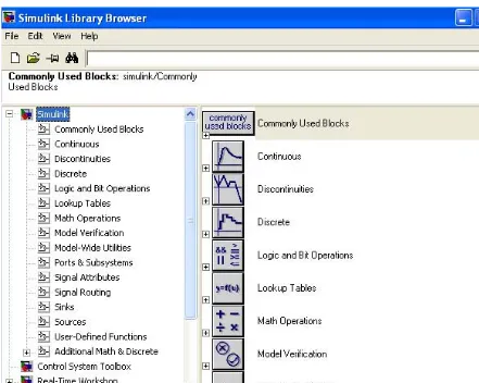
Upon execution of the Simulink command, the Commonly Used Blocks are shown in Figure 1.4.

In Figure 1.4, the left side is referred to as the Tree Pane and displays all Simulink libraries installed. The right side is referred to as the Contents Pane and displays the blocks that reside in the library currently selected in the Tree Pane.

Let us express the differential equation of Example 1.1 as

(1.26)

(25)

Chapter 1 Introduction to Simulink

Figure 1.4. The Simulink Library Browser

Figure 1.5. Block diagram for equation (1.26)

To model the differential equation (1.26) using Simulink, we perform the following steps:

1. On the Simulink Library Browser, we click the leftmost icon shown as a blank page on the top title bar. A new model window named untitled will appear as shown in Figure 1.6.

3

u₀( )t

Σ

∫

dt

∫

dt

−4

−3 d2vC

dt2

--- dvC dt

(26)

Figure 1.6. The Untitled model window in Simulink.

The window of Figure 1.6 is the model window where we enter our blocks to form a block dia-gram. We save this as model file name Equation_1_26. This is done from the File drop menu of Figure 1.6 where we choose Save as and name the file as Equation_1_26. Simulink will add the extension .mdl. The new model window will now be shown as Equation_1_26, and all saved files will have this appearance. See Figure 1.7.

Figure 1.7. Model window for Equation_1_26.mdl file

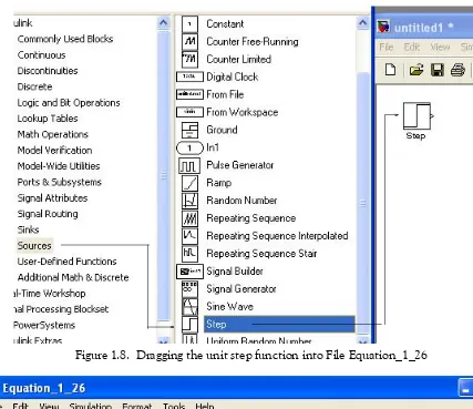
2. With the Equation_1_26 model window and the Simulink Library Browser both visible, we click the Sources appearing on the left side list, and on the right side we scroll down until we see the unit step function block shown as Step block. See Figure 1.8. We select it, and we drag it into the Equation_1_26 model window which now appears as shown in Figure 1.8. We save file Equation_1_26 using the File drop menu on the Equation_1_26 model window (right side of Figure 1.8).

3. With reference to block diagram of Figure 1.5, we observe that we need to connect an ampli-fier with Gain 3 to the unit step function block. The Gain block in Simulink is under Com-monly Used Blocks (first item under Simulink on the Simulink Library Browser). See Figure 1.8. If the Equation_1_26 model window is no longer visible, it can be recalled by clicking on the white page icon on the top bar of the Simulink Library Browser.

(27)

Chapter 1 Introduction to Simulink

Figure 1.8. Dragging the unit step function into File Equation_1_26

Figure 1.9. File Equation_1_26 with added Step and Gain blocks

5. Next, we need to add a thee−input adder. The adder block appears on the right side of the

Simulink Library Browser under Math Operations. We select it, and we drag it into the Equation_1_26 model window. We double click it, and on the Function Block Parameters

window which appears, we specify 3 inputs. We then connect the output of the Step block to the input of the Gain block, and the output of the of the Gain block to the first input of the

(28)

Figure 1.10. File Equation_1_26 with added Add block and connections between the blocks

6. From the Commonly Used Blocks of the Simulink Library Browser, we choose the Integra-tor block, we drag it into the Equation_1_26 model window, and we connect it to the output of the Add block. We repeat this step and to add a second Integrator block. We click the text “Integrator” under the first integrator block, and we change it to Integrator 1. Then, we change the text “Integrator 1” under the second Integrator to “Integrator 2” as shown in Fig-ure 1.11.

Figure 1.11. File Equation_1_26 with the addition of two integrators

7. To complete the model to represent the block diagram in Figure 1.5, we add the Scope block which is found in the Commonly Used Blocks on the Simulink Library Browser, we click the Gain block, and we copy and paste it twice. We flip the pasted Gain blocks by using the

Flip Block command from the Format drop menu, and we label these as Gain 2 and Gain 3. Finally, we double−click these gain blocks and in the Function Block Parameters dialog box, we change the gains in Gain 2 and Gain 3 blocks from unity to −4 and −3 as shown in Figure 1.12.

Figure 1.12. File Equation_1_26 complete block diagram

8. The initial conditions , and are entered by double− clicking the Integrator blocks and entering the values for the first integrator, and for the

iL 0

−

( ) CdvC dt

---t=0

0

= = v_c( )0− = 0.5 V

(29)

Chapter 1 Introduction to Simulink

double−click the Unit block and in the Source Block Parameters window we change the

Step time value from 1 to 0. We leave all other parameters in their default state. We also need to specify the simulation time. This is done by specifying the simulation time to be seconds on the Configuration Parameters from the Simulation drop menu. We can start the simula-tion on Start from the Simulation drop menu or by clicking the icon.

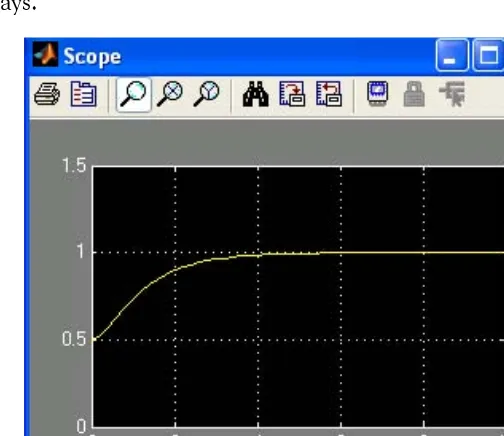
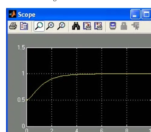
9. To see the output waveform, we double click the Scope block, and then clicking on the Autoscale icon. Then we right−click near the vertical axis, we click on Axes properties, we specify Y−min =0, Y−max = 1.5, we click OK, and we obtain the waveform shown in Fig-ure 1.13. Henceforth, we will use this procedFig-ure to scale the vertical axis in our subsequent

Scope block displays.

Figure 1.13. The waveform for the function in Example 1.1

Another easier method to obtain and display the output for Example 1.1, is to use State− Space block from Continuous in the Simulink Library Browser, as shown in Figure 1.14.

Figure 1.14. Obtaining the function for Example 1.1 with the State−Space block.

10

v_C( )t v_C( )t

(30)

The simout To Workspace block shown in Figure 1.14 writes its input to the workspace. In this example, we have assigned the name Example_1_1 to it, and Simulink appends it with the .mat

extension. As we know from our MATLAB studies, the data and variables created in the MAT-LAB Command window, reside in the MATMAT-LAB Workspace. This block writes its output to an array or structure that has the name specified by the block's Variable name parameter. It is highly recommended that this block is included in the saved model. This gives us the ability to delete or modify selected variables at a later time. To see what variables reside in the MATLAB Work-space, we issue the command who or whos.*

From Equation 1.23,

The output equation is or

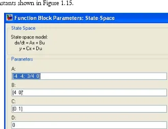
We double−click the State−Space block, and in the Functions Block Parameters window we enter the constants shown in Figure 1.15.

Figure 1.15. The Function block parameters for the State−Space block.

* who displays only the variables names, not the function to which each variable belongs. whos lists

(31)

Chapter 1 Introduction to Simulink

The initials conditions are specified at the MATLAB command prompt as x1=0; x2=0.5;

As before, to start the simulation we click the icon, and to see the output waveform, we dou-ble click the Scope block. Then we click on the Autoscale icon, and we scale the vertical axis as we did with the waveform of Figure 1.13. The waveform shown in Figure 1.16.

Figure 1.16. The waveform for the function for Example 1.1 with the State−Space block.

The state−space block is the best choice when we need to display the output waveform of three or more variables as illustrated by the following example.

Example 1.2

A fourth−order network is described by the differential equation

(1.27)

where is the output representing the voltage or current of the network, and is any input, and the initial conditions are .

a. We will express (1.27) as a set of state equations

(32)

b. It is known that the solution of the differential equation

(1.28)

subject to the initial conditions , has the solution

(1.29)

In our set of state equations, we will select appropriate values for the coefficients so that the new set of the state equations will represent the differential equa-tion of (1.28) and using Simulink, we will display the waveform of the output .

1. The differential equation of (1.28) is of fourth−order; therefore, we must define four state vari-ables that will be used with the four first−order state equations.

We denote the state variables as , and , and we relate them to the terms of the given differential equation as

(1.30)

We observe that

(1.31)

and in matrix form

(1.32)

In compact form, (1.32) is written as

(33)

Chapter 1 Introduction to Simulink

(1.35)

and since the output is defined as

relation (1.34) is expressed as

(1.36)

2. By inspection the differential equation of (1.27) will be reduced to the differential equation of (1.28) if we let

and thus the differential equation of (1.28) can be expressed in state−space form as

(1.37)

where

(1.38)

Since the output is defined as

in matrix form it is expressed as

(34)

(1.39)

We invoke MATLAB, we start Simulink by clicking on the Simulink icon, on the Simulink Library Browser, we click the Create a new model (blank page icon on the left of the top bar), and we save this model as Example_1_2. On the Simulink Library Browser we select

Sources, we drag the Signal Generator block on the Example_1_2 model window, we click and drag the State−Space block from the Continuous on Simulink Library Browser, and we click and drag the Scope block from the Commonly Used Blocks on the Simulink Library Browser. We also add the Display block found under Sinks on the Simulink Library Browser. We connect these four blocks and the complete block diagram is as shown in Figure 1.17.

Figure 1.17. Model for Example 1.2 with the entries specified below

We now double−click the Signal Generator block and we enter the following in the Function Block Parameters dialog box the following:

Wave form: sine

Time (t): Use simulation time Amplitude: 1

Frequency: 2 Units: Hertz

Next, we double−click the State−Space block and we enter the following parameter values in the Function Block Parameters:

(35)

Chapter 1 Introduction to Simulink

Now, we switch to the MATLAB Command window and at the command prompt we type the following values:

a0=1; a1=0; a2=2; a3=0; x0=[0 0 0 0]’;

We change the Simulation Stop time to , and we start the simulation by clicking on the icon. To see the output waveform, we double−click the Scope block, then we click the Autoscale icon, and we obtain the waveform shown in Figure 1.18.

Figure 1.18. Waveform for Example 1.2

The Display block in Figure 1.17 shows the value at the end of the simulation stop time.

Examples 1.1 and 1.2 have clearly illustrated that the State−Space is indeed a powerful block. We could have also obtained the solution of Example 1.2 using four Integrator blocks.

Example 1.3

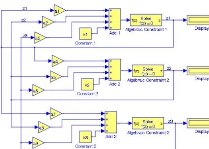
We will create a model that will produce the simultaneous solution of three equations with three unknowns using Algebraic Constraint blocks found in the Math Operations library, Display

blocks found in the Sinks library, and Gain blocks found in the Commonly Used Blocks library. The model will display the values for the unknowns , , and for the system of the equations

(1.40)

The model is shown in Figure 1.19.

25

z₁ z₂ z₃

(36)

Figure 1.19. Model for Example 1.3 with the entries specified below

Next, at the MATLAB command prompt we enter the following values: a1=2; a2=−3; a3=−1; a4=1; a5=5; a6=4; a7=−6; a8=1; a9=2;...

k1=−8; k2=−7; k3=5;

After clicking on the simulation icon, we obtain the values of the unknowns as , , and as shown in the Display blocks in Figure 1.19.

An Algebraic Constraint block constrains the input signal to zero, outputs a value for , and this value eventually produces a zero at the input. Thus, output is fed back to the input via a feedback path. We can improve the efficiency of the algebraic loop solver by providing an initial guess for the algebraic state that is close to the final solution value. By default, the initial guess value is zero.

An outstanding feature in Simulink is the representation of a large model consisting of many blocks and lines, to be shown as a single Subsystem block.

z₁ = 2 z₂ = –3 z₃ = 5

f z( ) z

(37)

Chapter 1 Introduction to Simulink

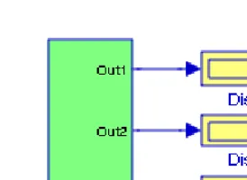
For instance, to group all blocks and lines in the model of Figure 1.19 except the display blocks, from the Edit drop menu we choose Create Subsystem and this model will be shown as in Figure 1.20* where at the MATLAB command prompt we have entered the following values:

a1=5; a2=−1; a3=4; a4=11; a5=6; a6=9; a7=−8; a8=4; a9=15;... k1=14; k2=−6; k3=9;

Figure 1.20. The model in Figure 1.19 represented as a subsystem

The Display blocks in Figure 1.20 show the values of , , and for the values that we speci-fied at the MATLAB command prompt above.

The Subsystem block is described in detail in Chapter 2, Section 2.1, Page 2−2.

1.2 Simulink Demos

At this time, the reader with no prior knowledge of Simulink, should be ready to learn Simulink’s additional capabilities. We will explore other features in the subsequent chapters. However, it is highly recommended that the reader becomes familiar with the block libraries found in the Sim-ulink Library Browser. Then, the reader can follow the steps delineated in The MathWorks Sim-ulink User’s Manual to run the Demo Models beginning with the thermo model. This model can invoked by typing thermo at the MATLAB command prompt.

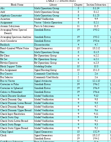
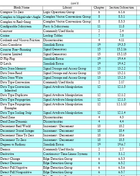
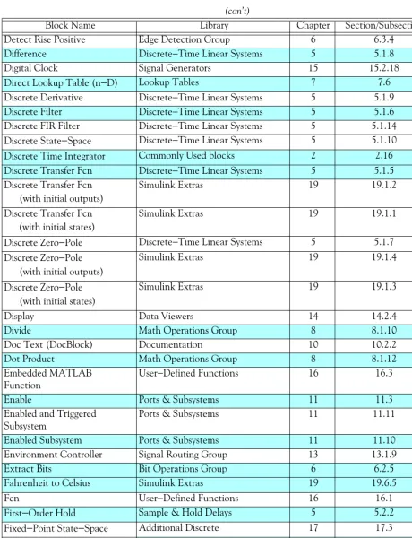
In the subsequent chapters, we will study each of the blocks under each of libraries in the Tree Pane. They are listed in Table 1.1 below in alphabetical order, the library where they appear, the chapter where they are described in this text, section/subsection, and page number in which they are described.

* The contents of the Subsystem block are not lost. We can double−click on the Subsystem block to see its con-tents. The Subsystem block replaces the inputs and outputs of the model with Inport and Outport blocks. These blocks along with the Subsystem block are described in Section 2.1, Chapter 2, Page 2−2.

(38)

TABLE 1.1 Simulink blocks

Block Name Library Chapter Section/Subsection Page

Abs Math Operations Group 8 8.1.14 8−10

Add Math Operations Group 8 8.1.2 8−2

Algebraic Constraint Math Operations Group 8 8.1.23 8−18

Assertion Model Verification 9 9.9 9−12

Assignment Vector / Matrix Operations 8 8.2.1 8−19 Atomic Subsystem Ports & Subsystems 11 11.5 11−4 Averaging Power Spectral

Density

Simulink Extras 19 19.3.2 19−37

Averaging Spectrum Analyzer Simulink Extras 19 19.3.2 19−41 Auto Correlator Simulink Extras 19 19.3.6 19−45

Backlash Discontinuities 4 4.7 4−9

Band−Limited White Noise Signal Generators 15 15.2.12 15−17

Bias Math Operations Group 8 8.1.5 8−4

Bit Clear Bit Operations Group 6 6.2.2 6−13

Bit Set Bit Operations Group 6 6.2.1 6−12

Bitwise Operator Bit Operations Group 6 6.2.3 6−14 Block Support Table Modeling Guides 10 10.3 10−9 Bus Assignment Signal Routing Group 13 13.1.3 13−2

Bus Creator Commonly Used blocks 2 2.6 2−8

Bus Selector Commonly Used blocks 2 2.6 2−8

(39)

Chapter 1 Introduction to Simulink

(con’t)

Block Name Library Chapter Section/Subsection Page Compare To Zero Logic Operations Group 6 6.1.6 6−9 Complex to Magnitude−Angle Complex Vector Conversions Group 8 8.3.1 8−26 Complex to Real−Imag Complex Vector Conversions Group 8 8.3.3 8−28 Configurable Subsystem Ports & Subsystems 11 11.8 11−19

Constant Commonly Used blocks 2 2.4 2−6

Cosine Lookup Tables 7 7.8 7−17

Coulomb and Viscous Friction Discontinuities 4 4.11 4−14 Cross Correlator Simulink Extras 19 19.3.5 19−43 Counter Free−Running Signal Generators 15 15.2.16 15−24 Counter Limited Signal Generators 15 15.2.15 15−25

D Flip Flop Simulink Extras 19 19.4.4 19−51

D Latch Simulink Extras 19 19.4.2 19−49

Data Store Memory Signal Storage and Access Group 13 13.2.2 13−19 Data Store Read Signal Storage and Access Group 13 13.2.1 13−18 Data Store Write Signal Storage and Access Group 13 13.2.3 13−19 Data Type Conversion Commonly Used blocks 2 2.17 2−32 Data Type Conversion

Inherited

Signal Attribute Manipulation 12 12.1.5 12−5

Data Type Duplicate Signal Attribute Manipulation 12 12.1.2 12−2 Data Type Propagation Signal Attribute Manipulation 12 12.1.3 12−4 Data Type Propagation

Examples

Signal Attribute Manipulation 12 12.1.10 12−14

Data Type Scaling Strip Signal Attribute Manipulation 12 12.1.4 12−5

Dead Zone Discontinuities 4 4.3 4−4

Dead Zone Dynamic Discontinuities 4 4.4 4−5

Decrement Real World Increment / Decrement 18 18.2 18−3 Decrement Stored Integer Increment / Decrement 18 18.4 18−5 Decrement Time To Zero Increment / Decrement 18 18.6 18−7 Decrement To Zero Increment / Decrement 18 18.5 18−6 Degrees to Radians Simulink Extras 19 19.6.7 19−65

Demux Commonly Used blocks 2 2.7 2−12

Derivative Continuous−Time Linear Systems 3 3.1.2 3−2 Detect Change Edge Detection Group 6 6.3.3 6−21 Detect Decrease Edge Detection Group 6 6.3.2 6−20 Detect Fall Negative Edge Detection Group 6 6.3.6 6−24 Detect Fall Nonpositive Edge Detection Group 6 6.3.7 6−25 Detect Increase Edge Detection Group 6 6.3.1 6−18 Detect Rise Nonnegative Edge Detection Group 6 6.3.5 6−23

(40)

(con’t)

Block Name Library Chapter Section/Subsection Page Detect Rise Positive Edge Detection Group 6 6.3.4 6−22 Difference Discrete−Time Linear Systems 5 5.1.8 5−9 Digital Clock Signal Generators 15 15.2.18 15−27 Direct Lookup Table (n−D) Lookup Tables 7 7.6 7−10 Discrete Derivative Discrete−Time Linear Systems 5 5.1.9 5−10 Discrete Filter Discrete−Time Linear Systems 5 5.1.6 5−5 Discrete FIR Filter Discrete−Time Linear Systems 5 5.1.14 5-19 Discrete State−Space Discrete−Time Linear Systems 5 5.1.10 5−11 DiscreteTime Integrator Commonly Used blocks 2 2.16 2−29 Discrete Transfer Fcn Discrete−Time Linear Systems 5 5.1.5 5−4 Discrete Transfer Fcn

(with initial outputs)

Simulink Extras 19 19.1.2 19-5

Discrete Transfer Fcn (with initial states)

Discrete Zero−Pole Discrete−Time Linear Systems 5 5.1.7 5−8 Discrete Zero−Pole

Discrete Zero−Pole (with initial states)

Display Data Viewers 14 14.2.4 14−16

Divide Math Operations Group 8 8.1.10 8−7

Doc Text (DocBlock) Documentation 10 10.2.2 10−9 Dot Product Math Operations Group 8 8.1.12 8−8 Embedded MATLAB

Function

User−Defined Functions 16 16.3 16−3

Enable Ports & Subsystems 11 11.3 11−2

Enabled and Triggered Subsystem

Ports & Subsystems 11 11.11 11−30

Enabled Subsystem Ports & Subsystems 11 11.10 11−27 Environment Controller Signal Routing Group 13 13.1.9 13−10 Extract Bits Bit Operations Group 6 6.2.5 6−17 Fahrenheit to Celsius Simulink Extras 19 19.6.5 19−63

Fcn User−Defined Functions 16 16.1 16−2

First−Order Hold Sample & Hold Delays 5 5.2.2 5−22 Fixed−Point State−Space Additional Discrete 17 17.3 17−4 Floating Bar Plot Simulink Extras 19 19.3.7 19−46

Floating Scope Data Viewers 14 14.2.2 14−8

For Iterator Subsystem Ports & Subsystems 11 11.13 11−37

From Signal Routing Group 13 13.1.13 13−14

(41)

Chapter 1 Introduction to Simulink

(con’t)

Block Name Library Chapter Section/Subsection Page From Workspace Models and Subsystems Inputs 15 15.1.4 15−2 Function−Call Generator Ports & Subsystems 11 11.4 11−3 Function−Call Subsystem Ports & Subsystems 11 11.12 11−34

Gain Commonly Used blocks 2 2.10 2−18

Goto Signal Routing Group 13 13.1.15 13−16

Goto Tag Visibility Signal Routing Group 13 13.1.14 13−15

Ground Commonly Used blocks 2 2.2 2−4

Hit Crossing Discontinuities 4 4.10 4−13

IC (Initial Condition) Signal Attribute Manipulation 12 12.1.6 12−6

If Ports & Subsystems 11 11.15 11−41

If Action Subsystem Ports & Subsystems 11 11.15 11−41 Increment Real World Increment / Decrement 18 18.1 18−2 Increment Stored Integer Increment / Decrement 18 18.3 18−4 Index Vector Signal Routing Group 13 13.1.7 13−8

Inport Commonly Used blocks 2 2.1 2−2

Integer Delay Discrete−Time Linear Systems 5 5.1.2 5−2

Integrator Commonly Used blocks 2 2.14 2−22

Interpolation (n−D) Using PreLookup

Lookup Tables 7 7.5 7−8

Interval Test Logic Operations Group 6 6.1.3 6−2 Interval Test Dynamic Logic Operations Group 6 6.1.4 6−3 J−K Flip Flop Simulink Extras 19 19.4.5 19−52 Level−2 M−File S−Function User−Defined Functions 16 16.5 16−7 Logical Operator Commonly Used blocks 2 2.12 2−20

Lookup Table Lookup Tables 7 7.1 7−2

Lookup Table (2−D) Lookup Tables 7 7.2 7−3

Lookup Table (n−D) Lookup Tables 7 7.3 7−6

Lookup Table Dynamic Lookup Tables 7 7.7 7−16 Magnitude−Angle to Complex Complex Vector Conversions Group 8 8.3.2 8−27 Manual Switch Signal Routing Group 13 13.1.10 13−12 Math Function Math Operations Group 8 8.1.16 8−11 MATLAB Fcn User−Defined Functions 16 16.2 16−3 Matrix Concatenate Vector / Matrix Operations 8 8.2.3 8−23

Memory Sample & Hold Delays 5 5.2.1 5−21

Merge Signal Routing Group 13 13.1.8 13−8

MinMax Math Operations Group 8 8.1.19 8−14

MinMax Running Resettable Math Operations Group 8 8.1.20 8−15

(42)

(con’t)

Model Ports & Subsystems 11 11.7 11−17

Model Info Documentation 10 10.2.1 10−7

Multiport Switch Signal Routing Group 13 13.1.11 13−13

Mux Commonly Used blocks 2 2.7 2−12

Outport Commonly Used blocks 2 2.1 2−2

Permute Math Operations Group 8 8.2.6 8−25

PID Controller Simulink Extras 19 19.2.6 19−29 PID Controller (with

approximate derivative)

Polar to Cartesian Simulink Extras 19 19.6.1 19−59 Polynomial Math Operations Group 8 8.1.18 8−14 Power Spectral Density Simulink Extras 19 19.3.1 19−33 Prelookup Index Search Lookup Tables 7 7.4 7−7 Probe Signal Attribute Detection 12 12.2.1 12−17

Product Commonly Used blocks 2 2.4 2−6

Product of Elements Math Operations Group 8 8.1.11 8−7 Pulse Generator Signal Generators 15 15.2.3 15−5

Quantizer Discontinuities 4 4.9 4−12

Radians to Degrees Simulink Extras 19 19.6.8 19−65

Ramp Signal Generators 15 15.2.5 15−9

Random Number Signal Generators 15 15.2.10 15−15

Rate Limiter Discontinuities 4 4.5 4−6

Rate Limiter Dynamic Discontinuities 4 4.6 4−8 Rate Transition Signal Attribute Manipulation 12 12.1.8 12−8 Real−Imag to Complex Complex Vector Conversions Group 8 8.3.4 8−29 Relational Operator Commonly Used blocks 2 2.11 2−19

Relay Discontinuities 4 4.8 4−11

Repeating Sequence Signal Generators 15 15.2.8 15−13 Repeating Sequence

Interpolated

Signal Generators 15 15.2.14 15−22

Repeating Sequence Stair Signal Generators 15 15.2.13 15−22 Reshape Vector / Matrix Operations 8 8.2.2 8−21 Rounding Function Math Operations Group 8 8.1.17 8−13 S−Function Ports & Subsystems

User−Defined Functions S−Function Builder User−Defined Functions 16 16.6 16−11 S−Function Examples User−Defined Functions 16 16.7 16−11

− −

(43)

Chapter 1 Introduction to Simulink

(con’t)

Block Name Library Chapter Section/Subsection Page Saturation Commonly Used blocks

Saturation Dynamic Discontinuities 4 4.2 4−3

Scope Data Viewers 14 14.2.1 14−6

Selector Signal Routing Group 13 13.1.6 13−6

Shift Arithmetic Bit Operations Group 6 6.2.4 6−16

Sign Math Operations Group 8 8.1.13 8−9

Signal Builder Signal Generators 15 15.2.4 15−6 Signal Conversion Signal Attribute Manipulation 12 12.1.7 12−7 Signal Generator Signal Generators 15 15.2.2 15−4 Signal Specification Signal Attribute Manipulation 12 12.1.9 12−11

Sine Lookup Tables 7 7.8 7−17

Sine Wave Signal Generators 15 15.2.6 15−9

Sine Wave Function Math Operations Group 8 8.1.22 8−17 Slider Gain Math Operations Group 8 8.1.8 8−6 Spectrum Analyzer Simulink Extras 19 19.33 19−38 Spherical to Cartesian Simulink Extras 19 19.6.3 19−61

Squeeze Math Operations Group 8 8.2.3 8−21

State−Space Continuous−Time Linear Systems 3 3.1.3 3−7 State−Space (with initial

outputs)

Step Signal Generators 15 15.2.7 15−12

Stop Simulation Simulation Control 14 14.3 14−17

Subsystem Commonly Used blocks 2 2.1 2−2

Subsystem Examples Ports & Subsystems 11 11.17 11−46

Subtract Math Operations Group 8 8.1.3 8−3

Sum Commonly Used blocks 2 2.9 2−17

Sum of Elements Math Operations Group 8 8.1.4 8−4

Switch Commonly Used blocks 2 2.8 2−15

Switch Case Ports & Subsystems 11 11.16 11−43 Switch Case Action Subsystem Ports & Subsystems 11 11.16 11−43 Switched Derivative for

Linearization

Switched Transport Delay for Linearization

Tapped Delay Discrete−Time Linear Systems 5 5.1.3 5−3

(44)

(con’t)

Terminator Commonly Used blocks 2 2.3 2−5

Time−Based Linearization Linearization of Running Models 10 10.1.2 10−4 To File Model and Subsystem Outputs 14 14.1.3 14−2 To Workspace Model and Subsystem Outputs 14 14.1.4 14−4 Transfer Fcn Continuous−Time Linear Systems 3 3.1.4 3−7 Transfer Fcn Direct Form II Additional Discrete 17 17.1 17−2 Transfer Fcn Direct Form II

Time Varying

Additional Discrete 17 17.2 17−3

Transfer Fcn First Order Discrete−Time Linear Systems 5 5.1.11 5−14 Transfer Fcn Lead or Lag Discrete−Time Linear Systems 5 5.1.12 5−15 Transfer Fcn Real Zero Discrete−Time Linear Systems 5 5.1.13 5−18 Transfer Fcn

Transfer Fcn

(with initial states)

Transport Delay Continuous−Time Delay 3 3.2.1 3−11

Trigger Ports & Subsystems 11 11.2 11−2

Trigger−Based Linearization Linearization of Running Models 10 10.1.1 10−2 Triggered Subsystem Ports & Subsystems 11 11.9 11−25 Trigonometric Function Math Operations Group 8 8.1.21 8−16 Unary Minus Math Operations Group 8 8.1.15 8−11 Uniform Random Number Signal Generators 15 15.2.11 15−16

Unit Delay Commonly Used blocks 2 2.15 2−27

Unit Delay Enabled Additional Discrete 17 17.7 17−9 Unit Delay Enabled

External IC

Unit Delay Enabled Resettable Additional Discrete 17 17.8 17−11 Unit Delay Enabled Resettable

External IC

Unit Delay External IC Additional Discrete 17 17.4 17−6 Unit Delay Resettable Additional Discrete 17 17.5 17−7 Unit Delay Resettable

External IC

Unit Delay With Preview Enabled

Unit Delay With Preview Enabled Resettable

Unit Delay With Preview Enabled Resettable External RV

(45)

Chapter 1 Introduction to Simulink

(con’t)

Block Name Library Chapter Section/Subsection Page Unit Delay With Preview

Resettable

Unit Delay With Preview Resettable External RV

Variable Time Delay Continuous−Time Delay 3 3.2.2 3−12 Variable Transport Delay Continuous−Time Delay 3 3.2.3 3−13 Vector Concatenate Vector / Matrix Operations 8 8.2.4 8−24 Weighted Sample Time Signal Attribute Detection 12 12.2.2 12−18 Weighted Sample Time Math Math Operations Group 8 8.1.6 8−5 While Iterator Subsystem Ports & Subsystems 11 11.14 11−39 Width Signal Attribute Detection 12 12.2.3 12−19

Wrap To Zero Discontinuities 4 4.12 4−16

XY Graph Data Viewers 14 14.2.3 14−12

Zero−Order Hold Sample & Hold Delays 5 5.2.3 5−23 Zero−Pole Continuous−Time Linear Systems 3 3.1.5 3−9 Zero−Pole (with initial outputs) Simulink Extras 19 19.2.4 19−26 Zero−Pole (with initial states) Simulink Extras 19 19.2.3 19−23

(46)

1.3 Summary

• MATLAB and Simulink are integrated and thus we can analyze, simulate, and revise our mod-els in either environment at any point. We invoke Simulink from within MATLAB.

• When Simulink is invoked, the Simulink Library Browser appears. The left side is referred to as the Tree Pane and displays all libraries installed. The right side is referred to as the Contents Pane and displays the blocks that reside in the library currently selected in the Tree Pane. • We open a new model window by clicking on the blank page icon that appears on the leftmost

position of the top title bar. On the Simulink Library Browser, we highlight the desired library in the Tree Pane, and on the Contents Pane we click and drag the desired block into the new model. Once saved, the model window assumes the name of the file saved. Simulink adds the extension .mdl.

• The > and < symbols on the left and right sides of a block are connection points.

• We can change the parameters of any block by double−clicking it, and making changes in the Function Block Parameters window.

• We can specify the simulation time on the Configuration Parameters from the Simulation

drop menu. We can start the simulation on Start from the Simulation drop menu or by click-ing on the icon. To see the output waveform, we double click on the Scope block, and then clicking on the Autoscale icon.

• It is highly recommended that the simout To Workspace block be added to the model so all data and variables are saved in the MATLAB workspace. This gives us the ability to delete or modify selected variables at a later time. To see what variables reside in the MATLAB Work-space, we issue the command who or whos.

• The state−space block is the best choice when we need to display the output waveform of three or more variables.

• We can use Algebraic Constrain blocks found in the Math Operations library, Display blocks found in the Sinks library, and Gain blocks found in the Commonly Used Blocks library, to draw a model that will produce the simultaneous solution of two or more equations with two or more unknowns.

(47)

Chapter 1 Introduction to Simulink

1.4 Exercises

1. Use Simulink with the Step function block, the Continuous−Time Transfer Fcn block, and the Scope block shown, to simulate and display the output waveform of the electric RLC circuit* shown below where is the unit step function, and the initial conditions are

, and .

2. Repeat Exercise 1 using integrator blocks in lieu of the transfer function block.

3. Repeat Exercise 1 using the State Space block in lieu of the transfer function block. 4. Using the State−Space block, create a model for the differential equation shown below.

subject to the initial conditions , and

* The electric circuits presented in this texts can be easily converted to their mechanical equivalent circuits where a voltage source can be replaced by a force f, a resistor can be replaced by a dashpot B, an inductor can be replaced by a mass M, and a capacitor can be replaced by an inverse spring constant 1/K. Thus the mechanical analog of the electric circuit above can be converted to the mechanical system shown below.

(48)

1.5 Solutions to End

−

of

−

Chapter Exercises

Dear Reader:

The remaining pages on this chapter contain solutions to all end−of−chapter exercises.

You must, for your benefit, make an honest effort to solve these exercises without first looking at the solutions that follow. It is recommended that first you go through and solve those you feel that you know. For your solutions that you are uncertain, look over your procedures for inconsistencies and computational errors, review the chapter, and try again. Refer to the solutions as a last resort and rework those problems at a later date.

(49)

Chapter 1 Introduction to Simulink

1.

The s−domain equivalent circuit is shown below.

and by substitution of the given circuit constants,

By the voltage division expression,

from which

We invoke Simulink from the MATLAB environment, we open a new file by clicking on the blank page icon at the upper left on the task bar, we name this file Exercise_1_1, and from the

Sources, Continuous, and Commonly Used Blocks in the Simulink Library Browser, we select and interconnect the desired blocks as shown below.

As we know, the unit step function is undefined at . Therefore, we double click the Step

block, and in the Source Block Parameters dialog box shown below we enter the values indi-cated. Likewise, we double click the Transfer Fcn block and in the Source Block Parameters

(50)

(51)

Chapter 1 Introduction to Simulink

On the model window, we click the Start Simulation icon and at the end of the simula-tion, we double−click the Scope block. The Scope block displays the waveform shown below after clicking the Autoscale icon. We observe that at the end of the simulation period (15 sec), the value across the capacitor is 0 and this is to be expected since at this time the inductor behaves as a short, thereby shorting the capacitor.

Let us compare the above waveform with that obtained with MATLAB using the plot com-mand. We want the output of the given circuit which we have defined as . The input is the unit step function whose Laplace transform is . Thus, in the complex frequency domain,

We obtain the Inverse Laplace transform of with the following MATLAB script: syms s

fd=ilaplace(1/(s^2+s+1))

v_out( )t = v_C( )t 1 s⁄

V_OUT( )s G s( )⋅V_IN( )s s s2+ +s 1 --- 1

s

---⋅ 1

s2+ +s 1

---= = =

(52)

fd = 2/3*3^(1/2)*exp(-1/2*t)*sin(1/2*3^(1/2)*t)

t=0.1:0.01:15; td=2./3.*3.^(1./2).*exp(−1./2.*t).*sin(1./2.*3.^(1./2).*t); plot(t,td); grid

The plot shown below is identical to that shown above which was obtained with Simulink.

2.

By Kirchoff’s Current Law (KCL),

By substitution of the circuit constants, observing that , and differentiating the above integro−differential equation, we obtain

(53)

Chapter 1 Introduction to Simulink

Invoking MATLAB, starting Simulink, and following the procedures of the examples and Exercise 1, we create the new model Exercise_1_2, shown below where for the Step block we specified Final value 0 to account for the fact that the final value across the capacitor will be zero since it will be shorted by the inductor. We double−click the Integrator 1 block and in the Function Block Parameters window we set the initial value to 0. We repeat this step for the Integrator 2 block and we also set the initial value to 0.

We start the simulation, and double−clicking the Scope block we obtain the graph shown below.

3.

We assign state variables x₁ and x₂ as shown below where x₁ = i_L and x₂ = v_C.

+

−

R

1 Ω _L

1 H

C

1 F − +

v_C

u₀t

i_R

i_C

(54)

Then,

and the initial conditions are

We form the model below and we name it Exercise_1_3.

(55)

Chapter 1 Introduction to Simulink

x0=[0 0]'; % This is a column vector

To avoid the unit step function discontinuity at , we double−click the Step block, and in the Source Block Parameters dialog box, we change the Initial value from 0 to 1.

The Display block shows the output value at the end of the simulation time, in this case 15. We click the Simulation start icon, we double−click the Scope block, and the output waveform is as shown below. We observe that this waveform is the same as in Exercises 1 and 2.

4.

subject to the initial conditions , and

We let and . Then, , and . Expressing the given equation as

we obtain the state−space equations

(56)

In matrix form,

subject to the initial conditions

Our simulation model is as shown below after specifying the conditions and values below.

1. We double−click the Sine Wave 1 block and in the Source Block Parameters dialog box we make the following entries:

Sine type: Time based

(57)

Chapter 1 Introduction to Simulink

2. We double−click the Sine Wave 2 block and in the Source Block Parameters dialog box we make the following entries:

Sine type: Time based

Time (t): Use simulation time Amplitude: −5

Bias: 0

Frequency (rad/sec): 2 Phase (rad): 5*pi/6 and we click OK

3. We double−click on the Signal Generator block and in the Source Block Parameters dia-log box we make the following entries:

Waveform: Sine

Time (t): Use external signal Amplitude: 1

Frequency: 2 (Hertz) and we click OK

4. We double−click on the State−Space block and in the Source Block Parameters dialog box we make the following entries:

A: [0 1; −1 −1], B=[1 0]’, C=[0 1], D=[0] Initial conditions: [x10 x 20]

and we click OK.

5. At the MATLAB command prompt we enter the initial conditions as x10=0; x20=0;

6. We click the Start Simulation icon, we double−click the Scope block, and after clicking the

(58)

(59)

Chapter 2 The Commonly Used Blocks Library

his chapter is an introduction to the Commonly Used Blocks Library. This is the first library in the Simulink group of libraries and contains the blocks shown below. In this chap-ter, we will describe the function of each block included in this library, and their application will be illustrated with examples.

T

(60)

2.1 The Inport, Outport, and Subsystem Blocks

Inport blocks are ports that serve as links from outside a system into the system. Outport blocks serve as links from the system to an outside system. A Subsystem block represents a subsystem of the system that contains it. As our model increases in size and complexity, we can simplify it by grouping blocks into subsystems. As we can see from Example 1.3 in Chapter 1, if we increase the number of the simultaneous equations, this model increases in size and complexity.

To create a subsystem before adding the blocks it will contain, we add a Subsystem block to the model, then we add the blocks that make up the subsystem. If the model already contains the blocks we want to convert to a subsystem, we create the subsystem by grouping the appropriate blocks. A Subsystem block can contain other subsystems.

Example 2.1

Figure 2.1 shows the model of Example 1.1, Figure 1.12 in Chapter 1. We will create a subsystem by grouping all blocks except the Step and the Scope blocks.

Figure 2.1. Model for Example 2.1

As a first step, we enclose the blocks and connecting lines that we want to include in the sub-system, within a bounding box. This is done by forming a rectangle around the blocks and the connecting lines to select them. Then, from the Edit drop menu we choose Create Subsystem

(61)

The Inport, Outport, and Subsystem Blocks

Figure 2.2. Model for Example 2.1 with Subsystem block

Next, we double−click the Subsystem block in Figure 2.2, and we observe that Simulink displays all blocks and interconnecting lines as shown in Figure 2.3 where the Step and Scope blocks in Figure 2.2, have been replaced by In1 and Out1 blocks respectively.

Figure 2.3. Model for Example 2.1 with Inport and Outport blocks replacing the Step and Scope blocks

The Inport (In1) and Outport (Out1) blocks represent the input to the subsystem and the output from the subsystem respectively. The Inport block name appears in the Subsystem icon as a port label. To suppress display of the label In1, we select the Inport block, we choose Hide Name from the Format menu, then choose Update Diagram from the Edit menu.

The Simulink demo F−14 Longitudinal Flight Control includes several Subsystem blocks. It can be accessed by typing sldemo_f14 at the MATLAB command prompt.

We can create any number of duplicates of an Inport block. The duplicates are graphical repre-sentations of the original intended to simplify block diagrams by eliminating unnecessary lines. The duplicate has the same port number, properties, and output as the original. Changing a dupli-cate's properties changes the original's properties and vice versa.

To create a duplicate of an Inport block, we select the block, we select Copy from the Simulink

Edit menu or from the block's context menu, we position the mouse cursor in the model's block diagram where we want to create the duplicate. and we select Paste Duplicate Inport from the Simulink Edit menu or the block diagram's context menu.

(62)

2.2 The Ground Block

The Ground block can be used to connect blocks whose input ports are not connected to other blocks. If we run a simulation with blocks having unconnected input ports, Simulink issues warn-ing messages. We can avoid the warnwarn-ing messages by uswarn-ing Ground blocks. Thus, the Ground block outputs a signal with zero value. The data type of the signal is the same as that of the port to which it is connected.

Example 2.2

Let us consider the model shown in Figure 2.4 where and and these values have been entered at the MATLAB command prompt. Upon execution of the Simulation start command, the sum of these two complex numbers is shown in the Display block.

Figure 2.4. Display of the sum of two complex numbers for Example 2.2

Next, let us delete the block with the value and execute the Simulation start command. The model is now shown as in Figure 2.5.

Figure 2.5. Model for Example 2.2 with Block K2 deleted.

Now, let us add a Ground block at the unconnected input of the Sum block and execute the Simulation start command. The model is now as shown in Figure 2.6.

K1 = 3+j1 K2 = 4+j3

(63)

The Terminator Block

Figure 2.6. Model of Figure 2.5 with a Ground block connected to the Sum block

More examples can be seen in the Bouncing Ball Demo model* by typing sldemo_bounce at the MATLAB command prompt, and in the Triggered Subsystem Demonstration model by typing triggeredsub at the MATLAB command prompt.

2.3 The Terminator Block

The Terminator block can be used to cap blocks whose output ports are not connected to other blocks. If we run a simulation with blocks having unconnected output ports, Simulink issues warning messages. We can avoid the warning messages by using Terminator blocks.

Example 2.3

Let us consider the unconnected output of the Product block in Figure 2.7 where the values for and are the same as in the previous example and are defined at the MATLAB command prompt.

Figure 2.7. Sum block with unconnected output for Example 2.3

When the simulation command is issued, the following message is displayed at the MATLAB Command Window:

* A similar demo is presented in Chapter 20.

(64)

Warning: Unconnected output line found on 'Figure_2_7R/Product' (output port: 1).

Figure 2.8 shows the Product block output connected to a Terminator block.

Figure 2.8. Sum block of Figure 2.7 with the Product block output connected to a Terminator block

For another example, refer to the Bouncing Ball Demo model by typing sldemo_bounce at the MATLAB command prompt.

2.4 The Constant and Product Blocks

The Constant block is used to define a real or complex constant value. This block accepts scalar (1x1 2−D array), vector (1−D array), or matrix (2−D array) output, depending on the dimension-ality of the Constant value parameter that we specify, and the setting of the Interpret vector parameters as 1−D parameter. The output of the block has the same dimensions and elements as the Constant value parameter. If we specify a vector for this parameter, and we want the block to interpret it as a vector (i.e., a 1−D array), we select the Interpret vector parameters as 1−D param-eter; otherwise, the block treats the Constant value parameter as a matrix (i.e., a 2−D array). By default, the Constant blockoutputs a signal whose data type and complexity are the same as that of the block's Constant value parameter. However, we can specify the output to be any sup-ported data type supsup-ported by Simulink, including fixed−point data types. For a discussion on the data types supported by Simulink, please refer to Data Types Supported by Simulink in the Using Simulink documentation.