Inverted Matrix: Efficient Discovery of Frequent Items in
Large Datasets in the Context of Interactive Mining
Mohammad El-Hajj
Department of Computing ScienceUniversity of Alberta Edmonton, AB, Canada, T6G 2E8
[email protected]
Osmar R. Za¨ıane
Department of Computing ScienceUniversity of Alberta Edmonton, AB, Canada, T6G 2E8
[email protected]
ABSTRACT
Existing association rule mining algorithms suffer from many problems when mining massive transactional datasets. One major problem is the high memory dependency: either the gigantic data structure built is assumed to fit in main ory, or the recursive mining process is too voracious in mem-ory resources. Another major impediment is the repetitive and interactive nature of any knowledge discovery process. To tune parameters, many runs of the same algorithms are necessary leading to the building of these huge data struc-tures time and again. This paper proposes a new disk-based association rule mining algorithm called Inverted Matrix, which achieves its efficiency by applying three new ideas. First, transactional data is converted into a new database layout called Inverted Matrix that prevents multiple scan-ning of the database during the miscan-ning phase, in which finding frequent patterns could be achieved in less than a full scan with random access. Second, for each frequent item, a relatively small independent tree is built summariz-ing co-occurrences. Finally, a simple and non-recursive min-ing process reduces the memory requirements as minimum candidacy generation and counting is needed. Experimental studies reveal that our Inverted Matrix approach outper-form FP-Tree especially in mining very large transactional databases with a very large number of unique items. Our random access disk-based approach is particularly advanta-geous in a repetitive and interactive setting.
Categories and Subject Descriptors
H.2.8 [Database Management]: Data Mining
Keywords
Association Rules, Frequent Patterns Mining, COFI-tree, Inverted Matrix
Permission to make digital or hard copies of all or part of this work for personal or classroom use is granted without fee provided that copies are not made or distributed for profit or commercial advantage and that copies bear this notice and the full citation on the first page. To copy otherwise, to republish, to post on servers or to redistribute to lists, requires prior specific permission and/or a fee.
SIGKDD ’03, August 24-27, 2003, Washington, DC, USA
Copyright 2003 ACM 1-58113-737-0/03/0008 ...$5.00.
1.
INTRODUCTION
Recent days have witnessed an explosive growth in gen-erating data in all fields of science, business, medicine, mil-itary, etc. The same rate of growth in the processing power of evaluating and analyzing the data did not follow this mas-sive growth. Due to this phenomenon, a tremendous volume of data is still kept without being studied. Data mining, a research field that tries to ease this problem, proposes some solutions for the extraction of significant and potentially use-ful patterns from these large collections of data. One of the canonical tasks in data mining is the discovery of associa-tion rules. Discovering associaassocia-tion rules, considered as one of the most important tasks, has been the focus of many studies in the last few years. Many solutions have been pro-posed using a sequential or parallel paradigm. However, the existing algorithms depend heavily on massive computation that might cause high dependency on the memory size or re-peated I/O scans for the data sets. Association rule mining algorithms currently proposed in the literature are not suf-ficient for extremely large datasets and new solutions, that do not depend on repeated I/O scans and less reliant on memory size, still have to be found.
1.1
Problem Statement
The problem of mining association rules over market bas-ket analysis was introduced in [1]. Association rules are not limited to market basket analysis, but the analysis of sales or what is known as basket data, is the typical application often used for illustration. The problem consists of find-ing associations between items or itemsets in transactional data. The data could be retail sales in the form of cus-tomer transactions or even medical images [14]. Association rules have been shown to be useful for other applications such as recommender systems, diagnosis, decision support, telecommunication, and even supervised classification [4]. Formally, as defined in [2], the problem is stated as follows: LetI ={i1, i2, ...im}be a set of literals, called items. m is
s% of the transactions inDcontainX∪Y. In other words, the support of the rule is the probability thatX andY hold together among all the possible presented cases. It is said that the rule X ⇒Y holds in the transaction set D with
confidence cifc% of transactions inDthat containX also containY. In other words, the confidence of the rule is the conditional probability that the consequentY is true under the condition of the antecedentX. The problem of discover-ing all association rules from a set of transactionsDconsists of generating the rules that have asupport and confidence
greater than a given threshold. These rules are calledstrong rules. This association-mining task can be broken into two steps: 1. A step for finding all frequentk-itemsets known for its extremeI/Oscan expense, and the massive computa-tional costs; 2. A straightforward step for generating strong rules.
1.2
Related Work
Several algorithms have been proposed in the literature to address the problem of mining association rules [10, 8]. One of the key algorithms, which seems to be the most popular in many applications for enumerating frequent itemsets is the
apriorialgorithm [2]. Thisapriorialgorithm also forms the foundation of most known algorithms. It uses a monotone property stating that for ak-itemset to be frequent, all its
k-1-itemsets have to be frequent. The use of this fundamen-tal property reduces the computational cost of candidate frequent itemsets generation. However, in the cases of ex-tremely large input sets with outsized frequent 1-items set, theapriori algorithm still suffers from two main problems of repeated I/O scanning and high computational cost. One major hurdle observed with most real datasets is the sheer size of the candidate frequent 2-itemsets and 3-itemsets. Park et al. have proposed the Dynamic Hashing and Prun-ing algorithm (DHP) [13]. This algorithm is also based on the monotoneapriori property, where a hash table is built for the purpose of reducing the candidate space by pre-computing the proximate support for thek+1 item set while counting thek-itemset. DHP has another important advan-tage, the transaction trimming, which removes the transac-tions that do not contain any frequent items. However this trimming and the pruning properties cause problems that make it impractical in many cases [16].
The partitioning algorithm proposed in [6] reduced the I/O cost dramatically. However, this method has problems in cases of high dimensional itemsets (i.e. large number of unique items), and it also suffers from the high false positives of frequent items. The Dynamic Itemset Counting (DIC) reduces the number of I/O passes by counting the candidates of multiple lengths in the same pass. DIC performs well in cases of homogenous data, while in other cases DIC might scan the databases more often than theapriori algorithm.
Another Innovative approach of discovering frequent pat-terns in transactional databases, FP-Growth, was proposed by Han et al. in [9]. This algorithm creates a compact tree-structure, FP-Tree, representing frequent patterns, that alleviates the multi-scan problem and improves the candi-date itemset generation. The algorithm requires only two full I/O scans of the dataset to build the prefix tree in main memory and then mines directly this structure. This special memory-based data structure becomes a serious bottleneck for cases with very large databases.
1.3
Motivations and Contributions
Apriori-like algorithms suffer from two main severe draw-backs: the extensive I/O scans for the databases, and the high cost of computations required for generating the fre-quent items. These drawbacks make these algorithms im-practical in cases of extremely large databases. Other algo-rithms like FP-Tree based depend heavily on the memory size as the memory size plays an important role in defining the size of the problem. Memory is not only needed to store the data structure itself, but also to generate recursively in the mining process a set of smaller trees called conditional trees. As argued by the authors of the algorithm, this is a serious constraint [12]. Other approaches such as in [11], build yet another data structure from which the FP-Tree is generated, thus doubling the need for main memory. One can argue that the tree structure, such as FP-tree, could be stored on disk. Indeed, using a B+tree, as suggested by the original authors of FP-growth, one could efficiently store the prefix tree. However, no one has really experimented this approach or reported on it. We have analyzed the use of a B+tree to store the FP-Tree and found out that the num-ber of I/Os increases significantly in the mining phase of the tree, defeating the purpose of building the tree structure in the first place.
The current association rule mining algorithms handle only relatively small sizes with low dimensions. Most of them scale up to only a couple of millions of transactions and a few thousands of dimensions [12, 7]. None of the exist-ing algorithms scales to beyond 15 million transactions, and hundreds of thousands of dimensions, in which each trans-action has an average of at least a couple of dozen items. This is the case for large businesses such as Walmart, Sears, UPS, etc.
In this paper we are introducing a new association rule mining disk-based algorithm that is based on the conditional pattern concept [9]. This algorithm is divided into two main phases. The first one, considered pre-processing, requires two full I/O scans of the dataset and generates a special disk-based data structure called Inverted Matrix. In the second phase, the Inverted Matrix is mined using different support levels to generate association rules using the Inverted Matrix algorithm explained later in this paper. The mining process might take in some cases less than one-full I/O scan of the data structure in which only frequent items based on the support given by the user are scanned and participate in generating the frequent patterns.
The reminder of this paper is organized as follows: Section 2 illustrates the transactional layout and the motivations of the Inverted Matrix approach. Section 3 describes the de-sign and constructions of the Co-Occurrence Frequent Item Trees. Section 4 depicts the Inverted Matrix algorithm. Ex-perimental results are given in Section 5. Finally, Section 6 concludes by discussing some issues and highlights our fu-ture work.
2.
TRANSACTION LAYOUT
2.1
Observations on Superfluous Processing
different values for the support threshold. In particular, if the support is consecutively reduced, k new scans of the database are needed for theapriori-based approaches, and a new memory structure is built for FP-growth like meth-ods. Notice that in each run of these algorithms, previous accumulated knowledge is not taken into account. For in-stance, in the simple transactional database of Figure 1A, where each line represents a transaction (called horizontal layout), we can observe that when changing support one can avoid reading some entries. If the support level is greater than 4, then Figure 1B highlights all frequent items that need to be scanned and computed. Non-circled items in Figure 1B are not included in the generation of the frequent items, and reading them becomes useless. It is known that all of the existing algorithms scan the whole database, fre-quent and non-frefre-quent items more than once generating a huge amount of useless work [12, 7, 8]. We call this super-fluous processing. Figure 1C represents what we actually need to read and compute from the transactional database based on a support greater than 4. Obviously, this may not be possible with this horizontal layout, but with a vertical layout avoiding these useless reads is possible.
T# Items
T1 A B C D E T2 A E C H G T3 B C D A E T4 F A H G J T5 A B C E I T6 K A E I C T7 A H E G I T8 K L M N O T9 L R Q A O T10 P N B A M
T# Items
T1 A B C D E T2 A E C H G T3 B C D A E T4 F A H G J T5 A B C E I T6 K A E I C T7 A H E G I T8 K L M N O T9 L R Q A O T10 P N B A M
T1 A C E T2 A E C T3 C A E T4 A T5 A C E T6 A E C T7 A E T9 A T10 A
T# Items
(A) (B) (C)
Figure 1: A: Transactional database (B): Frequent
items circled (C): Needed Items to be scanned,
σ >4.
The transaction layout is the method in which items in transactions are formatted in the database. Currently, there are two approaches: the horizontal approach and the vertical approach. In this section these approaches are discussed and a new transactional layout called Inverted Matrix is presented and compared with the existing two methods.
2.2
Horizontal vs. Vertical layout
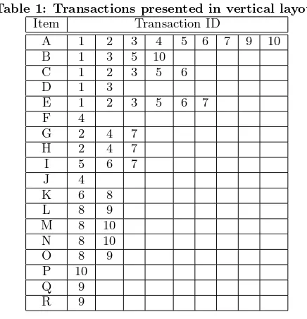
The relational database model consists of storing data into two-dimensional arrays called tables. Each table is made ofN rows called features or observations, and M columns called attributes or representing variables. The format of storing transactions in the database plays an important role in determining the efficiency of the association rule-mining algorithm used. Existing algorithms use one of the two lay-outs, namely horizontal and vertical. The first one, which is the most commonly used, relates all items on the same transaction together. In this approach the ID of the trans-action plays the role of the key for the transtrans-actional table. Figure 1A represents a sample of 10 transactions made of 18 items. The vertical layout relates all transactions that share the same items together. In this approach the key of each
Table 1: Transactions presented in vertical layout
Item Transaction ID
A 1 2 3 4 5 6 7 9 10 B 1 3 5 10
C 1 2 3 5 6
D 1 3
E 1 2 3 5 6 7 F 4
G 2 4 7
H 2 4 7
I 5 6 7 J 4
K 6 8
L 8 9
M 8 10 N 8 10
O 8 9
P 10 Q 9 R 9
record is the item. Each record in this approach has an item with all transaction numbers in which this item occurs. This is analogous to the idea of inverted index in information re-trieval where a word is associated with the set of documents it appears in. Here the word is an item and the document is a transaction. Transactions in Figure 1A are presented by using the vertical approach in Table 1. The horizontal layout has a very important advantage, which is combining all items in one transaction together. In this layout and by using some clever techniques, such as the one used in [9], the candidacy generation step can be eliminated. On the other hand, this layout suffers from limitations such as the prob-lem mentioned above that we called superfluous processing since there is no index on the items. The vertical layout, however, is an index on the items in itself and reduces the effect of large data sizes as there is no need to always re-scan the whole database. On the other hand, this vertical layout still needs the expensive candidacy generation phase. Also computing the frequencies of itemsets becomes the tedious task of intersecting records of different items of the candi-date patterns. In [15] a vertical database layout is combined with clustering techniques and hypergraph structures to find frequent itemsets. The candidacy generation and the addi-tional steps associated with this layout make it impractical for mining extremely large databases.
2.3
Inverted Matrix Layout
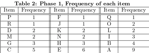
Table 2: Phase 1, Frequency of each item
Item Frequency Item Frequency Item Frequency
P 1 F 1 Q 1
R 1 J 1 O 2
D 2 K 2 L 2
M 2 N 2 I 3
G 3 H 3 B 4
C 5 E 6 A 9
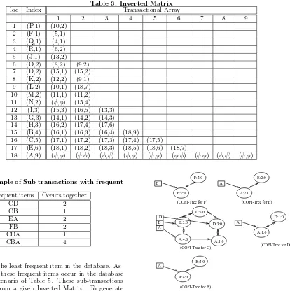
for the purpose of frequent itemset mining, it is discarded. The pointer is a pair where the first element indicates the address of a line in the matrix and the second element indi-cates the address of a column. Each line in the matrix has an address (sequential number in our illustrative example) and is prefixed by the item it represents with its frequency in the database. The lines are ordered in ascending order of the frequency of the item they represent. Table 3 repre-sents the Inverted Matrix corresponding to the transactional database from Figure 1A.
Building this Inverted Matrix is done in two phases, in which phase one scans the database once to find the fre-quency of each item and orders them into ascending order, such as in Table 2 for our illustrative example. The second phase scans the database again once to sort each transac-tion into ascending order according to the frequency of each item, and then fills in the matrix appropriately. To illustrate the process, let’s consider the construction of the matrix in Table 3. The first transaction in Figure 1A has items (A, B, C, D, E). This transaction is sorted into (D, B, C, E, A) based on the item frequencies in Table 2 built in the first phase of the process. Item D has the physical location line 7 in the Inverted Matrix in Table 3, B has the location line 15, the location of C is line 16, E is in line 17 and finally A is in line 18. This is according to the vertical approach. Item D has a link to the first empty slot in the transactional array of item B that is 1. Consequently, (15,1) entry is added in the first slot of item D to point to the first empty location in the transactional array of B. At the First empty location of B (15,1) an entry is added to point to the first empty location of the next item C that is (16,1). The same pro-cess occurs for all items in the transaction. The last item of the transaction, item A produces an entry with pointer null (φ,φ). The same is performed for every transaction.
Building the Inverted Matrix is assumed to be pre-processing of the transactional database. For a given transactional database, it is built once and for all. The next section presents an algorithm for mining association rules (or fre-quent itemsets) directly from this matrix. The basic idea is straight forward. For example, if the user decides to find all frequent patterns with support greater than 4, it suf-fices to start the mining process from location line 16. Line 16 represents the item C which has the frequency 5. Since the lines of the matrix are ordered, along with C, only the items that appear after C are frequent. All the other items are irrelevant for this particular support threshold. By fol-lowing in the Inverted Matrix the chain of items starting from the C location, we can rebuild parts of the transac-tions that contain only the frequent items. Thus, we avoid the superfluous processing mentioned before. Table 4 rep-resents the sub-transactions that can be generated from the Inverted Matrix of Table 3 by following the chains starting
from location line 16. The mining algorithm described in the next section targets these sub-transactions, and passes over all other parts dealing with de-facto non-frequent items. The sub-transactions of frequent items such as in Table 4 are never built at once. As will be explained in the next section, these sub-transactions are considered one frequent item at a time. In other words, using the Inverted Matrix, for each frequent item x, the algorithm would identify the sub-transactions of frequent items that contain x. These sub-transactions are then represented in a tree structure, that we call co-occurrence frequent item tree, which is mined individually.
Table 4: Sub-transactions with items having support
greater than 4. (A) List of sub-transactions; (B)
Condensed list.
C E A C E A C E A C E A C E A
C E A
(B) E A
5 1
Frequent Items Occurs
(A) E A
3.
CO-OCCURRENCE
FREQUENT-ITEM-TREES: DESIGN AND CONSTRUCTION
The generation of frequencies is considered a costly oper-ation for associoper-ation rule discovery. In apriori-based algo-rithms this step might become a complex problem in cases of high dimensionality due to the sheer size of the candi-dacy generation [8]. In methods such as FP-Growth [9], the candidacy generation is replaced by a recursive routine that builds a very large number of sub-trees, called conditional FP-trees, that are on the same order of magnitude as the fre-quent patterns and proved to be poorly scalable as attested by the authors [12].
Our approach for computing frequencies relies first on reading sub-transactions for frequent items directly from the Inverted Matrix, then building independent relatively small trees for each frequent item in the transactional database. We mine separately each one of the trees as soon as they are built, with minimizing the candidacy generation and with-out building conditional sub-trees recursively. The trees are discarded as soon as mined.
The small trees we build (Co-Occurrence Frequent Item Tree, or COFI-Tree for short) are similar to the conditional FP-tree in general in the sense that they have a header with ordered frequent items and horizontal pointers point-ing to a succession of nodes containpoint-ing the same frequent item, and the prefix tree per-se with paths representing sub-transactions. However, the COFI-trees have bidirectional links in the tree allowing bottom-up scanning as well, and the nodes contain not only the item label and a frequency counter, but also a participation counter as explained later in this section. Another difference, is that a COFI-tree for a given frequent itemxcontains only nodes labeled with items that are more frequent or as frequent asx.
Table 3: Inverted Matrix
loc Index Transactional Array
1 2 3 4 5 6 7 8 9
1 (P,1) (10,2) 2 (F,1) (5,1) 3 (Q,1) (4,1) 4 (R,1) (6,2) 5 (J,1) (13,2) 6 (O,2) (8,2) (9,2) 7 (D,2) (15,1) (15,2) 8 (K,2) (12,2) (9,1) 9 (L,2) (10,1) (18,7) 10 (M,2) (11,1) (11,2) 11 (N,2) (φ,φ) (15,4)
12 (I,3) (15,3) (16,5) (13,3) 13 (G,3) (14,1) (14,2) (14,3) 14 (H,3) (16,2) (17,4) (17,6)
15 (B,4) (16,1) (16,3) (16,4) (18,9)
16 (C,5) (17,1) (17,2) (17,3) (17,4) (17,5)
17 (E,6) (18,1) (18,2) (18,3) (18,5) (18,6) (18,7)
18 (A,9) (φ,φ) (φ,φ) (φ,φ) (φ,φ) (φ,φ) (φ,φ) (φ,φ) (φ,φ) (φ,φ)
Table 5: Example of Sub-transactions with frequent items
Frequent items Occurs together
CD 2
CB 1
EA 2
FB 2
CDA 1
CBA 4
item, and F is the least frequent item in the database. As-sume also that these frequent items occur in the database following the scenario of Table 5. These sub-transactions are generated from a given Inverted Matrix. To generate the frequent 2-itemsets, theapriorialgorithm would need to generate 15 different patterns out of the 6 items{A, B, C, D, E, F}. Finding the frequency of each pattern and removing the non-frequent ones is necessary before even considering the candidate 3-itemsets. In our approach, itemsets of dif-ferent sizes are found simultaneously. In particular, for each given frequent 1-itemset we find all frequent k-itemsets that subsume it. For this, a COFI-tree is built for each frequent item except the most frequent one, starting from the least frequent. No tree is built for the most frequent item since by definition a COFI-tree of an itemxcontains items that are more frequent thanx.
With our example, the first Co-Occurrence Frequent Item tree is built for item F. In this tree for F, all frequent items which are more frequent than F and share transactions with F participate in building the tree. The tree starts with the root node containing the item in question, F. For each sub-transaction containing item F with other frequent items that are more frequent than F, a branch is formed starting from the root node F. If multiple frequent items share the same prefix, they are merged into one branch and a account for each node of the tree is adjusted accordingly. Figure 2 il-lustrates all COFI-trees for frequent items of Table 5. In
E:2:0
B D B
(COFI-Tree for F)
A:1:0 (COFI-Tree for E)
(COFI-Tree for B)
D:1:0 B:2:0
F:2:0
A:2:0
B:4:0
(COFI-Tree for C) (COFI-Tree for D) C:8:0
B:5:0
A:4:0
D:3:0
A:1:0
A:4:0
A
A
A
A
Figure 2: COFI-Trees
Figure 2, the round nodes are nodes from the tree with an item label and two counters. The first counter is a support for that node while the second counter, called participation-count, is initialized to 0 and is used by the mining algorithm discussed later. The nodes have also pointers: a horizontal link which points to the next node that has the same item-namein the tree, and a bi-directional vertical link that links a child node with its parent and a parent with its child. The bi-directional pointers facilitate the mining process by mak-ing the traversal of the tree easier. The squares are actually cells from the header table as with the FP-Tree. This is a list made of all frequent items that participate in building the tree structure sorted in ascending order of their global support. Each entry in this list contains theitem-nameand a pointer to the first node in the tree that has the same item-name.
only with item B in the database presented in Table 5. The same thing happens with item E, but it occurs with item A twice. Item C occurs with 3 items, namely A, B and D, and consequently 4 nodes are created as CBA: 4 forms one branch with support = 4 for each node in the branch. CDA: 1 creates another branch with support =1 for the branch except node C as its support becomes 5 (4+1). Pattern CD: 2 already has a branch built, so only the frequency is updated, C becomes 7, and D becomes 3. Finally CB: 1 already shares the same prefix with an existing branch so only counters are updated and thus C becomes 8 and B becomes 5. The D tree is made of one branch as item D occurs once with an item that is more frequent than D, which is in DA: 1 in CDA: 1. Finally item B occurs 4 times with item A from CBA: 4 (C is ignored in the last two cases as it is less frequent than B and A). The header in each tree, like with FP-Trees, constitutes a list of all frequent items to maintain the location of first entry for each item in the COFI-Tree. A link is also made for each node in the tree that points to the next location of the same item in the tree if it exists.
The COFI-trees of all frequent items are not constructed together. Each tree is built, mined, then discarded before the next COFI-tree is built. The mining process is done for each tree independently with the purpose of finding all frequent k-itemset patterns that the item on the root of the tree participates in. A top-down approach is used to gen-erate and compute maximumn patterns at a time, where
n is the number of nodes in the COFI-tree that is being mined excluding the root node of the tree. The frequency of other sub-patterns can be deduced from their parent pat-terns without counting their occurrences in the database.
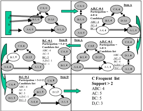
Steps to produce frequent patterns related to the C item for example, are illustrated in Figure 3. From each branch of the tree, using the support count and the participation count, candidate frequent patterns are identified and stored temporarily in a list. The non-frequent ones are discarded at the end when all branches are processed. Figure 3 shows the frequent itemsets containing C discovered assuming a support threshold greater than 2. Mining the “COFI-tree of item C” starts from the most frequent item in the tree, which is item A. Item A exists in two branches in the C tree which are (A: 4, B: 5, and C:8) and (A: 1, D: 3, and C: 8). The frequency of each branch is the frequency of the first item in the branch minus the participation value of the same node. Item A in the first branch has a frequency value of 4 and participation value of 0 which makes the first pattern ABC frequency equals to 4. The participations values for all nodes in this branch are incremented by 4, which is the frequency of this pattern. In the first pattern ABC: 4, we need to generate all sub patterns that item C participates in which are AC: 4 and BC: 4. The second branch that has A generates the pattern ADC: 1 as the frequency of A on this branch is 1 and its participation value equals to 0. All participation values on these nodes is incremented by 1. Sub-patterns are also generated from the ADC pattern which are DC: 1 and AC: 1. The second pattern already exists with support value equals to 4, and only updating its value is needed to make it equal to 5. The second frequent item in this tree, “B” exists in one branch (B: 5 and C: 5) with participation value of 4 for the B node. (BC: 1) is pro-duced from this branch and since BC pattern already exists with a frequency value equals to 4, then only its frequency is
updated to become 5. Finally, the D item is the last item to test as it exists in one branch, (D: 3, C: 8) with participation value of 1 for the D node. A pattern DC: 2 is produced and its value is added to the existing DC: 1 pattern to make it DC: 3. Finally all non-frequent patterns are omitted leaving us with only frequent patterns that item C participate in. The COFI-Tree of Item C can be removed at this time and another tree can be generated and tested to produce all the frequent patterns related to the root node.
D
Figure 3: Steps needed to generate frequent pat-terns related to item C
4.
INVERTED MATRIX ALGORITHM
The Inverted Matrix association rule algorithms are sets of algorithms with the purpose of mining large transactional databases with minimal candidacy generation and reducing the effects of superfluous work. These algorithms are divided among the two phases of the mining process namely the pre-processing in which the Inverted Matrix is built and the mining phase in which the discovery of frequent patterns occurs.
4.1
Building the Inverted Matrix
second item the same process occurs, in which an entry in the transactional table of the second item is added to hold the location of the third item in the transaction. The same process is repeated for all items in this transaction. The following transaction is read next and the same occurs for all its items. This process repeats for all transactions in the database. Algorithm 1 depicts the steps needed to build the Inverted Matrix.
Algorithm 1: Inverted Matrix (IM) Construction
Input : Transactional Database (D)
Output :Disk Based Inverted Matrix
Method : Pass I
1. ScanDto identify unique items with their frequencies. 2. Sort the items in ascending order of their frequency. 3. Create the index part of the IM using the sorted list.
Pass II
1. While there is a transactionT in the database (D) do
1.1 Sort the items in the transactionT into ascending order according to their frequency
1.2 while there are itemssiin the transaction do
1.2.1 Add an entry in its corresponding
transactional array row with 2- parameters (A) Location in index part of the IM of the
next itemsi+1 inT nullifsi+1does not
exist.
(B) Location of the next empty slot in the transactional array row ofsi+1,nullifsi+1
does not exist. 1.3 Goto 1.2
2. Goto 1
4.2
Mining the Inverted Matrix
Association rule mining starts by defining the support levelσ. Based on the given support, the algorithm finds all frequent patterns that occur more thanσ. The objectives behind the Inverted Matrix mining algorithm are two fold: first, minimizing the candidacy generation; second, eliminat-ing the superfluous scans of non-frequent items. To accom-plish this, asupport borderis defined. This border indicates where to slice the Inverted Matrix to gain direct access to those items that are frequent. In other words, the border is the first item in the index of the Inverted matrix that has a support greater or equal to σ. For Each item I in the index of the slice of the inverted matrix is considered at a time starting from the least frequent, a Co-Occurrence Frequent Item Tree forI is built by following the chain of pointers in the transactional array of the Inverted Matrix. ThisI-COFI-tree is mined branch by branch starting with the node of the most frequent item and going upward in the tree to identify candidate frequent patterns containingI. A list of these candidates is kept and updated with frequencies of the branches where they occur. Since a node could belong to more than one branch of the tree, a participation count is used to avoid re-counting items and patterns. Algorithm 2 presents the steps needed to generate the COFI-trees and mining them.
Algorithm 2: Creating and Mining COFI-Trees
Input: Inverted Matrix (IM) and a minimum support thresh-oldσ
Output: Full set of frequent patterns
Method:
1. Frequency Location = Apply binary search on the index part of the IM to find the Location of the first frequent item based onσ.
2. While (Frequency Location<IM Size) do 2.1 A = Frequent item at
location (Frequency Location)
2.2 A Transactional = The Transactional array of item A
2.3 Create a root node for the (A)-COFI-Tree with
frequency-count andparticipation-count = 0 2.4 Index Of TransactionalArray = 0
2.5 While (Index Of TransactionalArray<Frequency of item A)
2.5.1 B = item from Transactional array at location (Index Of TransactionalArray)
2.5.2 Follow the chain of item B to produce sub-transaction C
2.5.3 Items on C form a prefix of the (A)-COFI-Tree. 2.5.4 If the prefix is new then
2.5.4.1 Setfrequency-count= 1 and participation-count= 0 for all nodes in the path
. Else
2.5.4.2 Adjust thefrequency-count of the already exist part of the path.
2.5.5 Adjust the pointers of theHeader listif needed 2.5.6 Increment Index Of TransactionalArray 2.5.7 Goto 2.5
2.6 MineCOFI-Tree (A) 2.7 Release (A) COFI-Tree
2.8 Increment Frequency Location //to build the next COFI-Tree
3. Goto 2
Function: MineCOFI-Tree (A)
1. nodeA = select next node //Selection of nodes will start with the node of most frequent item and following its chain, then the next less frequent item with its chain, until we reach the least frequent item in theHeader list of the (A)-COFI-Tree
2. while there are still nodes do
2.1 D = set of nodes from nodeA to the root 2.2 F=frequency-count-participation-count of nodeA 2.3 Generate all Candidate patterns X from
items in D. Patterns that do not have A will be discarded
2.4 Patterns in X that do not exist in the A-Candidate List will be added to it with frequency = F otherwise just increment their frequency with F 2.5 Increment the value ofparticipation-count
by F for all items in D 2.6 nodeA = select next node 2.7 Goto 2
3. Based on support thresholdσremove non-frequent patterns from A Candidate List.
the transactional array for item C denotes that it shares the same transaction with the item at location 17 which is E. At location (17,1) we find that the other item A at location 18, shares with them the same transaction. From this, the first child node of C is created holding an entry for item E, and another child node from E is created holding an entry for item A. The frequency of all these items are set to 1 and their participation is set to 0. The second entry of the transactional array of item C is (17,2), and at location (17,2) we find an entry of (18,2). This means that items E, and A also share another transaction with item C. Since entries for these items have already been created in the same order, then there will be no need to create new nodes as we will only increment their frequencies. By scanning all entries for item C with their chain, we can build the C-COFI-Tree as in Figure 4A. Methods in Algorithm 2 are applied on the C-COFI-Tree to generate all frequent patterns related to C, which are CE:5, CA:5, and CEA:5. The C-COFI-Tree can be released at this stage, and its memory space can be used for the next tree.
C:5:0
A:5:0 A E
(A)
A
A:6:0 E:6:0
(B) E:5:0
Figure 4: COFI-Trees (A) Item C, (B) Item E
The same process happens for the next frequent item that is at location 17 (item E). Figure 4B presents its COFI-Tree which generates the frequent pattern EA:6.
5.
EXPERIMENTAL EVALUATIONS AND
PERFORMANCE STUDY
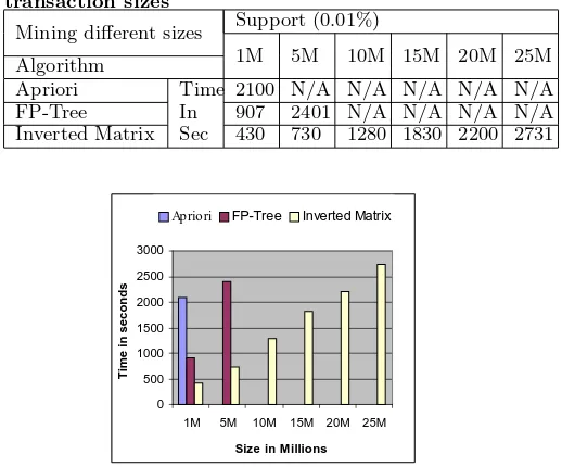
To test the efficiency of the Inverted Matrix approach, we conducted experiments comparing our approach with a two well-known algorithms namely:Aprioriand FP-Growth. To avoid implementation bias, third partyApriori implementa-tion, by Christian Borgelt [5], and FP-growth [9] written by its original authors are used. The experiments were run on a 733-Mhz machine with a relatively small RAM of 256MB. Transactions were generated using IBM synthetic data generator [3]. We conducted different experiments to test the Inverted Matrix algorithm when mining extremely large transactional databases. We tested the applicability and scalability of the Inverted Matrix algorithm. In one of these experiments, we mined using a support threshold of 0.01% transactional databases of sizes ranging from 1 million to 25 million transactions with an average transaction length of 24 items. The dimensionality of the 1 million transaction dataset was 10,000 items while the datasets ranging from 5 million to 25 million transactions had a dimensionality of 100,000 unique items. Table 6 and Figure 5 illustrate the comparative results obtained withApriori, FP-Growth and the Inverted Matrix. Apriori failed to mine the 5 million transactional database and FP-Tree couldn’t mine beyond the 5 million transaction mark. The Inverted Matrix,
how-ever, demonstrates good scalability as this algorithm mines 25 million transactions in 2731s (about 45 min). None of the tested algorithms, or reported results in the literature reaches such a big size.
Table 6: Time needed in seconds to mine different transaction sizes
Mining different sizes Support (0.01%)
1M 5M 10M 15M 20M 25M Algorithm
Apriori Time 2100 N/A N/A N/A N/A N/A FP-Tree In 907 2401 N/A N/A N/A N/A Inverted Matrix Sec 430 730 1280 1830 2200 2731
0 500 1000 1500 2000 2500 3000
1M 5M 10M 15M 20M 25M
Size in Millions
Time in seconds
Apriori FP-Tree Inverted Matrix
Figure 5: Time needed in seconds to mine different transaction sizes
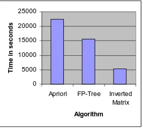
To test the behavior of the Inverted Matrix vis-`a-vis differ-ent support thresholds, a set of experimdiffer-ents was conducted on a database size of one million transactions, with 10,000 items and an average transaction length of 24 items. The matrix was built in about 763 seconds and it occupied a size of 109MB on the hard drive. The original transactional database with a horizontal layout uses 102MB. The mining process tested different support levels, which are 0.0025% that revealed almost 125K frequent patterns, 0.005% that revealed nearly 70K frequent patterns, 0.0075% that gen-erated 32K frequent patterns and 0.01 that returned 17K frequent patterns. Table 7 reports the time needed in sec-onds for each one of these runs. The results show that the Inverted Matrix algorithm outperforms both Apriori and FP-growth algorithms in all cases. Figure 6 depicts the re-sults of Table 7. It is true that there was an overhead cost which was not recorded in Table 7, namely the cost of build-ing the Inverted Matrix. In this particular reported result we meant to focus on the actual mining time. The Inverted Matrix is built once for all and used to mine with four differ-ent support thresholds. The total execution time needed for FP-Growth to mine these four cases is 15607s, whileApriori
Notice that given the highly interactive nature of most KDD processes, a “build-once-mine-many” approach is always de-sirable.
Table 7: Time needed to mine 1M transactions with different supports level
Mining 1M transactions Support (%)
0.0025 0.005 0.0075 0.01 Algorithm
Apriori Time 11300 6200 2900 2100 FP-Tree In 6800 5600 2300 907 Inverted Matrix Sec. 2300 1030 780 430
0 2000 4000 6000 8000 10000 12000
0.01 0.0075 0.005 0.0025 Support (%)
Time in seconds
Apriori FP-Tree Inverted Matrix
Figure 6: Time needed to mine 1M transactions with different supports levels
0 5000 10000 15000 20000 25000
Apriori FP-Tree Inverted Matrix
Algorithm
Time in second
s
Figure 7: Accumulated time needed to mine 1M transactions using four different support levels
6.
DISCUSSION AND FUTURE WORK
Finding scalable algorithms for association rule mining in extremely large databases is the main goal of our research. To reach this goal, we propose a new set of algorithms that uses the disk to store the transactions in a special layout called Inverted Matrix. It also uses the memory to inter-actively mine relatively small structures called COFI-Trees. The experiments we conducted showed that our algorithms are scalable to mine tens of millions of transactions, if not more. Our study reinforces that in mining extremely large transactions; we should not work on algorithms that build huge memory data structures, nor on algorithms that scan the massive transactions many times. What we need is a
disk-based-algorithm that can store the massive size and al-low random access, and small memory structures that can be independently created and mined based on the available absolute memory size.
While the results seem promising, there are still many im-provements that can be done to further develop the Inverted Matrix approach. We are currently focusing on building a parallel framework for association rule mining for large-scale data that would use the matrix idea in a cluster context. The improvements we are currently investigating are issues related to the reduction of the Inverted Matrix size (i.e. compression), the reduction of the number of I/Os when building the COFI-trees, the update of the matrix by addi-tion and deleaddi-tion of transacaddi-tions, and the parallelizaaddi-tion of the construction and mining of the Inverted Matrix.
6.1
Compressing the size of Inverted Matrix
Compressing the size of the Inverted Matrix without los-ing any data is an important issue that could improve the efficiency of the Inverted Matrix algorithm. To achieve this, one could merge similar transactions into new dummy ones, or even merge sub-transactions. For example in Figure 1A, we can find that the first two transactions contain items A, B, C, D, E and A, E, C, H, G. Ordering both transactions as usual into ascending order according to their frequency pro-duces two new transactions, which are D, B, C, E, A and G, H, C, E, A. Both transactions share the same suffix, which is C, E, and A. Consequently, we can view them as one trans-action consisting ofD,B
G,H(C(2), E(2), A(2)), where any
num-ber between brackets represents the occurrences of the item preceding it. Using the same methodology we can find that the Inverted Matrix can be compressed. The compressed Inverted Matrix corresponding to Figure 1A is depicted in Table 8. With such compressed matrix we can dramatically reduce the number of I/Os and thus improve further the performance.
Table 8: Compressed Inverted Matrix
loc Index Transactional Array
1 2 3
1 (P,1) (10,2)(1) 2 (F,1) (5,1)(1) 3 (Q,1) (4,1)(1) 4 (R,1) (6,2)(1) 5 (J,1) (13,2)(1)
6 (O,2) (8,2)(1) (9,2)(1) 7 (D,2) (15,1)(2)
8 (K,2) (12,2)(1) (9,1)(1) 9 (L,2) (10,1)(1) (18,1)(1) 10 (M,2) (11,1)(1) (11,2)(1) 11 (N,2) (φ,φ)(1) (15,2)(1)
12 (I,3) (15,1)(1) (16,1)(1) (13,3)(1) 13 (G,3) (14,1)(1) (14,2)(2)
14 (H,3) (16,1)(1) (17,1)(2) 15 (B,4) (16,1)(3) (18,1)(1) 16 (C,5) (17,1)(5)
6.2
Reducing the number of I/Os needed
The Inverted Matrix groups the transactions based on their frequency. Frequent items are clustered at the bot-tom of the Inverted Matrix. Traversing one transaction can be done by calling more than one page from the database. We are currently investigating the possibility of reducing the number of pages read from the database by clustering the same transactions on the same pages at the database level.
6.3
Updateable Inverted Matrix
With a horizontal layout, adding transactions is simply appending those transactions to the database. With a ver-tical layout, each added transaction results in updates in the database entries of all items in the transaction. The Inverted Matrix is neither horizontal nor vertical but a combination, making the addition of new transactions a complex opera-tion. Updateable Inverted Matrix is an important issue in our research. One of the main advantages of the Inverted Matrix is that changing the support level does not mean re-scanning the database again. Changing the database ei-ther by adding or deleting transactions changes the Inverted Matrix, leading to the need of re-building it again. We are investigating efficient ways to update the Inverted Matrix without having to rebuild it completely or jeopardizing its integrity.
6.4
Parallelizing the Inverted Matrix
The Inverted Matrix could be built in parallel. Each pro-cessor could build its own Inverted Matrix that reflects all transactions on its node in the cluster. The index part of the small Inverted Matrices would reflect the global frequency of the items in all transactions. Building these distributed Inverted Matrices would also be done using two passes over the local data. The first pass or scan to generate the local frequency for each item. Generating the global frequency of each item could be done either by broadcasting or scattering these local supports. The second pass for each local node is almost identical to the second pass of the sequential ver-sion, where communication between nodes is minimal. Min-ing the distributed Inverted Matrices would start by findMin-ing the support border based on the given support by the user. Each node creates its conditional pattern for each item and sends it to a designated processor for the said item to gen-erate its global conditional pattern, which in turn elicits the frequent patterns.
7.
ACKNOWLEDGMENTS
We would like the thank Jian Pei for providing us with the executable code of the FP-Growth program used in our experiments. This research is partially supported by a Re-search Grant from NSERC, Canada.
8.
REFERENCES
[1] R. Agrawal, T. Imielinski, and A. Swami. Mining association rules between sets of items in large databases. InProc. 1993 ACM-SIGMOD Int. Conf. Management of Data, pages 207–216, Washington, D.C., May 1993.
[2] R. Agrawal and R. Srikant. Fast algorithms for mining association rules. InProc. 1994 Int. Conf. Very Large Data Bases, pages 487–499, Santiago, Chile,
September 1994.
[3] IBM. Almaden. Quest synthetic data generation code. http://www.almaden.ibm.com/cs/quest/syndata.html. [4] M.-L. Antonie and O. R. Za¨ıane. Text document
categorization by term association. InIEEE International Conference on Data Mining, pages 19–26, December 2002.
[5] C. Borgelt. Apriori implementation.
http://fuzzy.cs.uni-magdeburg.de/~borgelt/apriori/apriori.html. [6] S. Brin, R. Motwani, J. D. Ullman, and S.Tsur.
Dynamic itemset counting and implication rules for market basket data. InProc. 1997 ACM-SIGMOD Int. Conf. Management of Data, pages 255–264, Tucson, Arizona, May 1997.
[7] E.-H. Han, G. Karypis, and V.Kumar. Scalable parallel data mining for association rule.Transactions on Knowledge and data engineering, 12(3):337–352, May-June 2000.
[8] J. Han and M. Kamber.Data Mining: Concepts and Techniques. Morgan Kaufman, San Francisco, CA, 2001.
[9] J. Han, J. Pei, and Y. Yin. Mining frequent patterns without candidate generation. InACM-SIGMOD, Dallas, 2000.
[10] J. Hipp, U. Guntzer, and G. Nakaeizadeh. Algorithms for association rule mining - a general survey and comparison.ACM SIGKDD Explorations, 2(1):58–64, June 2000.
[11] H. Huang, X. Wu, and R. Relue. Association analysis with one scan of databases. InIEEE International Conference on Data Mining, pages 629–636, December 2002.
[12] J. Liu, Y. Pan, K. Wang, and J. Han. Mining frequent item sets by oppotunistic projection. In Eight ACM SIGKDD Internationa Conf. on Knowledge Discovery and Data Mining, pages 229–238, Edmonton, Alberta, August 2002.
[13] J. Park, M. Chen, and P. Yu. An effective hash-based algorithm for mining association rules. InProc. 1995 ACM-SIGMOD Int. Conf. Management of Data, pages 175–186, San Jose, CA, May 1995.
[14] O. R. Za¨ıane, J. Han, and H. Zhu. Mining recurrent items in multimedia with progressive resolution refinement. InInt. Conf. on Data Engineering (ICDE’2000), pages 461–470, San Diego, CA, February 2000.
[15] M. Zaki, S. Parthasarathy, M. Ogihara, and W. Li. New algorithms for fast discovery of association rules. In3rd Intl. Conf. on Knowledge Discovery and Data Mining, 1997.