Penilaian Asset & Bisnis
PROGRAM STUDI AKUNTANSI
FAKULTAS EKONOMI DAN BISNIS
UNIVERSITAS ESA UNGGUL
EBA 919
PENILAIAN
ASSET & BISNIS
1 Damodaran
Valuing Equity in
Firms in Distress
Aswath Damodaran
2 Damodaran
The Going Concern Assumption
Traditional valuation techniques are built on the assumption of a going
concern, I.e., a firm that has continuing operations and there is no significant threat to these operations.
• In discounted cashflow valuation, this going concern assumption finds its place most prominently in the terminal value calculation, which usually is based upon an infinite life and ever-growing cashflows.
• In relative valuation, this going concern assumption often shows up implicitly because a firm is valued based upon how other firms - most of which are healthy - are priced by the market today.
When there is a significant likelihood that a firm will not survive the
immediate future (next few years), traditional valuation models may yield an over-optimistic estimate of value.
∑
(1 + WACC) ttValue of Firm =
3 Damodaran
Valuing a Firm
The value of the firm is obtained by discounting expected cashflows to
the firm, i.e., the residual cashflows after meeting all operating expenses and taxes, but prior to debt payments, at the weighted
average cost of capital, which is the cost of the different components
of financing used by the firm, weighted by their market value proportions. t= n
CF to Firm
t =1
where,
CF to Firmt = Expected
Cashflow to Firm in period t
WACC = Weighted Average Cost of Capital
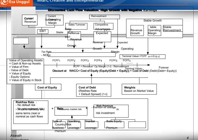
Discounted Cash Flow Valuation: High Growth with Negative Earnings
Margin
...
Discount at WACC= Cost of Equity (Equity/(Debt + Equity)) + Cost of Debt (Debt/(Debt+ Equity))
4 Damodaran
Beta
risk investment - No reinvestment risk
Stable Growth
Revenue Operating Reinvestment Growth Margin
Terminal Value= FCFF n+1/(r-g n)
Current
Revenue Operating
EBIT
Revenue Expected
Discounted Cash Flow Valuation: High Growth with Negative
Current Reinvestment Current Operating
Sales Turnover Competitive
Ratio Advantages Stable S
EBIT Revenue
Revenue Expected
Growth
Growth Operating
Tax Rate Margin - NOLs
FCFF = Revenue* Op Margin (1-t) - Reinvestment
Terminal Value=
table Stable
Forever Value of Operating Assets
+ Cash & Non-op Assets = Value of Firm
- Value of Debt = Value of Equity - Equity Options
= Value of Equity in Stock
FCFF1 FCFF2 FCFF3 FCFF4 FCFF5 FCFFn
Discount at WACC= Cost of Equity (Equity/(Debt + Equity)) + Cost of Debt
Cost of Equity Cost of Debt
(Riskfree Rate
+ Default Spread) (1-t)
Weights
Based on Market Value
Riskfree Rate :
- No default risk Risk Premium - In same currency and + - Measures market risk X - Premium for average in same terms (real or
nominal as cash flows
Type of Operating Financial Base Equity Country Risk
Business Leverage Leverage Premium Premium
=$ 28,683
1 2 3 4 5 6 7 8 9 10
Cost of Equity 16.80% 16.80% 16.80% 16.80% 16.80% 15.20% 13.60% 12.00% 10.40% 8.80%
Cost of Capital 13.80% 13.80% 13.80% 13.80% 13.80% 12.92% 11.94% 10.88% 9.72% 7.98%
Debt= 74.91% -> 40%
November 2001 5 Damodaran Stable Growth 30% ROC=7.36% 67.93%
Terminal Value= 677(.0736-.05)
$13,902
Revenue Margin:
-1895m Revenue EBITDA/Sales
2,076m
Current Current
Revenue Margin: Stable $ 3,804 -49.82% Cap ex growth slows
and net cap ex Stable Stable decreases Revenue EBITD
EBIT Growth: 5% Sales
Growth: -> 30%
NOL: 13.33%
2,076m Terminal Value=
Revenues $3,804 $5,326 $6,923 $8,308 $9,139 $10,053 $11,058 $11,942 $12,659 $13,292
EBITDA ($95) $ 0 $346 $831 $1,371 $1,809 $2,322 $2,508 $3,038 $3,589
EBIT ($1,675) ($1,738) ($1,565) ($1,272) $320 $1,074 $1,550 $1,697 $2,186 $2,694
EBIT (1-t) ($1,675) ($1,738) ($1,565) ($1,272) $320 $1,074 $1,550 $1,697 $2,186 $2,276
+ Depreciation $1,580 $1,738 $1,911 $2,102 $1,051 $736 $773 $811 $852 $894
- Cap Ex $3,431 $1,716 $1,201 $1,261 $1,324 $1,390 $1,460 $1,533 $1,609 $1,690
- Chg WC $ 0 $46 $48 $42 $25 $27 $30 $27 $21 $19
Stable
A/ Reinvest
Term. Year
$ 4,187 $ 3,248 $ 2,111 $ 939 $ 2,353 $ 20 $ 677
Forever
Value of Op Assets $ 5,530
+ Cash & Non-op $ 2,260 = Value of Firm $ 7,790 - Value of Debt $ 4,923 = Value of Equity $ 2867 - Equity Options $ 14 Value per share $ 3.22
FCFF ($3,526) ($1,761) ($903) ($472) $22 $392 $832 $949 $1,407 $1,461
Beta 3.00 3.00 3.00 3.00 3.00 2.60 2.20 1.80 1.40 1.00
Cost of Debt 12.80% 12.80% 12.80% 12.80% 12.80% 11.84% 10.88% 9.92% 8.96% 6.76% Debt Ratio 74.91% 74.91% 74.91% 74.91% 74.91% 67.93% 60.95% 53.96% 46.98% 40.00%
Cost of Equity
16.80% Cost of Debt4.8%+8.0%=12.8% Tax rate = 0% -> 35%
Weights
Riskfree Rate:
T. Bond rate = 4.8% Risk Premium
Beta 4%
+ 3.00> 1.10 X
Internet/ Operating Current Base Equity Country Risk Retail Leverage D/E: 441% Premium Premium
Global Crossing
Stock price = $1.86
6 Damodaran
I. Discount Rates:Cost of Equity
Preferably, a bottom-up beta, based upon other firms in the business, and firm’s own financial leverage
Cost of Equity = Riskfree Rate + Beta * (Risk Premium)
Has to be in the same Historical Premium Implied Premium
currency as cash flows, 1. Mature Equity Market Premium: Based on how equity and defined in same terms Average premium earned by or market is priced today (real or nominal) as the stocks over T.Bonds in U.S. and a simple valuation cash flows 2. Country risk premium = model
Country Default Spread* ( σEquity/σCountry bond)
7 Damodaran 20 00 19 98 19 96 19 94 19 92 19 90 19 88 19 86 19 84 19 82 19 80 19 78 19 76 19 74 19 72 19 70 19 68 19 66 19 64 19 62 19 60 Im pl ie d P re m iu m
Implied Premium for US Equity Market
8 Damodaran
Beta Estimation: Global Crossing
j =k Operating Income
j
Firm
j =1
= βunlevered[1 + (1 − tax rate) (Current Debt/Equity Ratio) ]
βlevered
9 Damodaran
The Solution: Bottom-up Betas
The bottom up beta can be estimated by :
• Taking a weighted (by sales or operating income) average of the unlevered betas of the different businesses a firm is in.
jOperating Income
(The unlevered beta of a business can be estimated by looking at other firms in the same business)
• Lever up using the firm’s debt/equity ratio
The bottom up beta will give you a better estimate of the true beta
when
• It has lower standard error (SEaverage = SEfirm / √n (n = number of firms)
• It reflects the firm’s current business mix and financial leverage • It can be estimated for divisions and private firms.
10 Damodaran
Global Crossing’s Bottom-up Beta
Unlevered beta for firms in telecommunications equiipment = 0.752 Current market debt to equity ratio = 298.56%
Levered beta for Global Crossing = 0.752 ( 1+ (1-0) (2.9856)) = 3.00
Global Crossing’s current market values of debt and equity are used to
compute the market debt to equity ratio.
• Market value of equity = Price/share * # shares = $ 1.86 * 886.47 = $1,649 million
• Market value of debt = 415 (PV of Annuity, 12.80%, 8 years) + 7647/1.1288 =
$4,923 million
( $ 407 million = Interest expenses; $7,647 = Book value of debt; 8 years = Average debt maturity and 12.8% is the pre-tax cost of debt)
Global Crossing pays no taxes and is not expected to pay taxes for 9 years…
Marginal tax rate, reflecting (1) synthetic or actual bond rating
Weights should be market value weights based upon bottom-up
11 Damodaran
From Cost of Equity to Cost of Capital
Cost of borrowing should be based upon
(2) default spread tax benefits of debt
Cost of Borrowing = Riskfree rate + Default spread
Cost of Capital = Cost of Equity (Equity/(Debt + Equity)) + Cost of Borrowing (1-t) (Debt/(Debt + Equity))
Cost of equity
beta
12 Damodaran
Interest Coverage Ratios, Ratings and Default
Spreads
If Interest Coverage Ratio is Estimated Bond Rating Default Spread(1/01)
> 8.50 AAA 0.75%
6.50 - 8.50 AA 1.00%
5.50 - 6.50 A+ 1.50%
4.25 - 5.50 A 1.80%
3.00 - 4.25 A- 2.00%
2.50 - 3.00 BBB 2.25%
2.00 - 2.50 BB 3.50%
1.75 - 2.00 B+ 4.75%
1.50 - 1.75 B 6.50%
1.25 - 1.50 B - 8.00% 0.80 - 1.25 CCC 10.00%
0.65 - 0.80 CC 11.50%
0.20 - 0.65 C 12.70%
< 0.20 D 15.00%
13 Damodaran
Estimating the cost of debt for a firm
The rating for Global Crossing is B- and the default spread is 8%. Adding this
to the T.Bond rate in November 2001 of 4.8% Pre-tax cost of debt = Riskfree Rate + Default spread
= 4.8% + 8.00% = 12.80%
After-tax cost of debt = 12.80% (1- 0) = 12.80%: The firm is paying no taxes
currently. As the firm’s tax rate changes and its cost of debt changes, the after tax cost of debt will change as well.
1 2 3 4 5 6 7 8 9 10 Pre-tax 12.80% 12.80% 12.80% 12.80% 12.80% 11.84% 10.88% 9.92% 8.96% 8.00%
Tax rate 0% 0% 0% 0% 0% 0% 0% 0% 0% 16% After-tax 12.80% 12.80% 12.80% 12.80% 12.80% 11.84% 10.88% 9.92% 8.96% 6.76%
14 Damodaran
Estimating Cost of Capital: Global Crossing
Equity
• Cost of Equity = 4.80% + 3.00 (4.00%) = 16.80%
• Market Value of Equity = $ 1.86 * 886.47 = $1,649 million (25.09%)
Debt
• Cost of debt = 4.80% + 8% (default spread) = 12.80% • Market Value of Debt = $ 4,923 mil (74.91%)
Cost of Capital
Cost of Capital = 16.8 % (.2509) + 12.8% (1- 0) (.7491)) = 13.80%
- Tax rate * EBIT
= EBIT ( 1- tax rate)
- (Capital Expenditures - Depreciation)
- Change in non-cash working capital
15 Damodaran
- R&D
Defined as
- Non-debt CL - can be effective for
move to marginal
operating losses
II. Estimating Cash Flows to Firm
Operating leases R&D Expenses
- Convert into debt - Convert into asset
- Adjust operating income - Adjust operating income
Update Normalize Cleanse operating items of
- Trailing Earnings - History - Financial Expenses - Unofficial numbers - Industry - Capital Expenses
- Non-recurring expenses
Earnings before interest and taxes
Tax rate
near future, but
- reflect net
Non-cash CA
Include = Free Cash flow to the firm (FCFF)
- Acquisitions
16 Damodaran
The Importance of Updating
The operating income and revenue that we use in valuation should be updated
numbers. One of the problems with using financial statements is that they are dated.
As a general rule, it is better to use 12-month trailing estimates for earnings
and revenues than numbers for the most recent financial year. This rule becomes even more critical when valuing companies that are evolving and growing rapidly.
Last 10-K Trailing 12-month
Revenues $ 3,789 million $3,804 million EBIT -$1,396 million - $ 1,895 million Depreciation $1,381 million $1,436 million Interest expenses $ 390 million $ 415 million Debt (Book value) $ 7,271 million $ 7,647 million Cash $ 1,477 million $ 2,260 million
17 Damodaran
Estimating FCFF: Global Crossing
EBIT (Trailing 2001) = -$ 1,895 million
Tax rate used = 0% (
Capital spending (Trailing 2001) = $4,289 million
Depreciation (Trailing 2001) = $ 1,436 million
Non-cash Working capital Change (2001) = - 63 million
Estimating FCFF (Trailing 12 months)
Current EBIT * (1 - tax rate) = - 1895 (1-0) = - $ 1,895 million - (Capital Spending - Depreciation) = $ 2,853 million - Change in Working Capital = -$ 63 million Current FCFF = - $ 4,685 million
Global Crossing funded a significant portion of this cashflow by selling assets (ILEC) for about $3.4 billion.
18 Damodaran
IV. Expected Growth in EBIT and
Fundamentals
Reinvestment Rate and Return on Capital
gEBIT = (Net Capital Expenditures + Change in WC)/EBIT(1-t) *
ROC= Reinvestment Rate * ROC
Proposition: No firm can expect its operating income to grow over
time without reinvesting some of the operating income in net capital expenditures and/or working capital.
Proposition: The net capital expenditure needs of a firm, for a given
growth rate, should be inversely proportional to the quality of its investments.
19 Damodaran
Revenue Growth and Operating Margins
With negative operating income and a negative return on capital, the
fundamental growth equation is of little use for Global Crossing.
For Global Crossing, the effect of reinvestment shows up in revenue
growth rates and changes in expected operating margins, but with a lagged effect.
We will assume that Global Crossing’s cap ex growth will slow and
that depreciation lags cap ex by about 3 years.
20 Damodaran
Cap Ex and Depreciation: Global Crossing
Year Cap Ex Cap Ex Growth Depreciation epreciation Growt Net Cap ex 1 $3,431 -20.00% $1,580 10.00% $1,852
2 $1,716 -50.00% $1,738 10.00% -$22
3 $1,201 -30.00% $1,911 10.00% -$710
4 $1,261 5.00% $2,102 10.00% -$841
5 $1,324 5.00% $1,051 -50.00% $273
6 $1,390 5.00% $736 -30.00% $654
7 $1,460 5.00% $773 5.00% $687
8 $1,533 5.00% $811 5.00% $721
9 $1,609 5.00% $852 5.00% $758 10 $1,690 5.00% $894 5.00% $795
Stable Growth 2-Stage Growth 3-Stage Growth
21 Damodaran
V. Growth Patterns
A key assumption in all discounted cash flow models is the period of
high growth, and the pattern of growth during that period. In general, we can make one of three assumptions:
• there is no high growth, in which case the firm is already in stable growth • there will be high growth for a period, at the end of which the growth rate will drop to the stable growth rate (2-stage)
• there will be high growth for a period, at the end of which the growth rate will decline gradually to a stable growth rate(3-stage)
22 Damodaran
Stable Growth Characteristics
In stable growth, firms should have the characteristics of other stable
growth firms. In particular,
• The risk of the firm, as measured by beta and ratings, should reflect that of a stable growth firm.
- Beta should move towards one
- The cost of debt should reflect the safety of stable firms (BBB or higher)
• The debt ratio of the firm might increase to reflect the larger and more stable earnings of these firms.
- The debt ratio of the firm might moved to the optimal or an industry average - If the managers of the firm are deeply averse to debt, this may never happen
• The reinvestment rate of the firm should reflect the expected growth rate and the firm’s return on capital
- Reinvestment Rate = Expected Growth Rate / Return on Capital
23 Damodaran
Global Crossing: Stable Growth Inputs
High Growth Stable Growth
Global Crossing
• Beta 3.00 1.00 • Debt Ratio 74.9% 40% • Return on Capital Negative 7.36% • Cost of capital 13.80% 7.36% • Expected Growth Rate NMF 5%
• Reinvestment Rate >100% 5%/7.36% = 67.93%
24 Damodaran
Why distress matters…
Some firms are clearly exposed to possible distress, though the source of
the distress may vary across firms.
• For some firms, it is too much debt that creates the potential for failure to make debt payments and its consequences (bankruptcy, liquidation,
reorganization)
• For other firms, distress may arise from the inability to meet operating expenses.
When distress occurs, the firm’s life is terminated leading to a
potential loss of all cashflows beyond that point in time.
• In a DCF valuation, distress can essentially truncate the cashflows well before you reach “nirvana” (terminal value).
• A multiple based upon comparable firms may be set higher for firms that have continuing earnings than for one where there is a significant chance that these earnings will end (as a consequence of bankruptcy).
25 Damodaran
The Purist DCF Defense: You do not need to
consider distress in valuation
If we assume that there is unrestricted access to capital, no firm that is
worth more as a going concern will ever be forced into liquidation.
• Response: But access to capital is not unrestricted, especially for firms that are viewed as troubled and in depressed financial markets.
The firms we value are large market-cap firms that are traded on major
exchanges. The chances of these firms defaulting is minimal…
• Response: Enron and Kmart….
Firms that default will be able to sell their assets (both in-place and
growth opportunities) for a fair market value, which should be equal to the expected operating cashflows on these assets.
• Response: Unlikely, even for assets-in-place, because of the need to liquidate quickly.
26 Damodaran
The Adapted DCF Defense: It is already in the
valuation
The expected cashflows can be adjusted to reflect the likelihood of
distress. For firms with a significant likelihood of distress, the expected cashflows should be much lower.
• Response: Easier said than done. Most DCF valuations do not consider the likelihood in any systematic way. Even if it is done, you are implicitly
assuming that in the event of distress, the distress sale proceeds will be equal to the present value of the expected cash flows.
The discount rate (costs of equity and capital) can be adjusted for the
likelihood of distress. In particular, the beta (or betas) used to estimate the cost of equity can be estimated using the updated debt to equity ratio, and the cost of debt can be increased to reflect the current default risk of the firm.
• Response: This adjusts for the additional volatility in the cashflows but not for the truncation of the cashflows.
27 Damodaran
Dealing with Distress in DCF Valuation
Simulations: You can use probability distributions for the inputs into
DCF valuation, run simulations and allow for the possibility that a string of negative outcomes can push the firm into distress.
Modified Discounted Cashflow Valuation: You can use probability
distributions to estimate expected cashflows that reflect the likelihood of distress.
Going concern DCF value with adjustment for distress: You can value
the distressed firm on the assumption that the firm will be a going concern, and then adjust for the probability of distress and its consequences.
Adjusted Present Value: You can value the firm as an unlevered firm
and then consider both the benefits (tax) and costs (bankruptcy) of debt.
28 Damodaran
I. Monte Carlo Simulations
Preliminary Step: Define the circumstances under which you would
expect a firm to be pushed into distres.
Step 1: Choose the variables in the DCF valuation that you want
estimate probability distributions on.
Steps 2 & 3: Define the distributions (type and parameters) for each of
these variables.
Step 4: Run a simulation, where you draw one outcome from each
distribution and compute the value of the firm. If the firm hits the “distress conditions”, value it as a distressed firm.
Step 5: Repeat step 4 as many times as you can.
Step 6: Estimate the expected value across repeated simulations.
29 Damodaran
II. Modified Discounted Cashflow Valuation
If you can come up with probability distributions for the cashflows
(across all possible outcomes), you can estimate the expected cash flow in each period. This expected cashflow should reflect the
likelihood of default. In conjunction with these cashflow estimates, you should estimate the discount rates by
• Using bottom-up betas and updated debt to equity ratios (rather than historical or regression betas) to estimate the cost of equity
• Using updated measures of the default risk of the firm to estimate the cost of debt.
If you are unable to estimate the entire distribution, you can at least
estimate the probability of distress in each period and use as the expected cashflow:
Expected cashflowt = Cash flowt * (1 - Probability of distresst)
30 Damodaran
III. DCF Valuation + Distress Value
A DCF valuation values a firm as a going concern. If there is a
significant likelihood of the firm failing before it reaches stable growth and if the assets will then be sold for a value less than the present
value of the expected cashflows (a distress sale value), DCF valuations will understate the value of the firm.
Value of Equity= DCF value of equity (1 - Probability of distress) +
Distress sale value of equity (Probability of distress)
31 Damodaran
Step 1: Value the firm as a going concern
You can value a firm as a going concern, by looking at the expected
cashflows it will have if it follows the path back to financial health. The costs of equity and capital will also reflect this path. In particular, as the firm becomes healthier, the debt ratio (which is high at the time of the distress) will converge to more normal levels. This, in turn, will lead to lower costs of equity and debt.
Most discounted cashflow valuations, in my view, are implicitly going
concern valuations.
=$ 28,683
1 2 3 4 5 6 7 8 9 10
Cost of Equity 16.80% 16.80% 16.80% 16.80% 16.80% 15.20% 13.60% 12.00% 10.40% 8.80%
Cost of Capital 13.80% 13.80% 13.80% 13.80% 13.80% 12.92% 11.94% 10.88% 9.72% 7.98%
Debt= 74.91% -> 40%
November 2001 32 Damodaran Stable Growth 30% ROC=7.36% 67.93%
Terminal Value= 677(.0736-.05)
$13,902
Revenue Margin:
-1895m Revenue EBITDA/Sales
2,076m
Current Current
Revenue Margin: Stable $ 3,804 -49.82% Cap ex growth slows
and net cap ex Stable Stable decreases Revenue EBITD
EBIT Growth: 5% Sales
Growth: -> 30%
NOL: 13.33%
2,076m Terminal Value=
Revenues $3,804 $5,326 $6,923 $8,308 $9,139 $10,053 $11,058 $11,942 $12,659 $13,292
EBITDA ($95) $ 0 $346 $831 $1,371 $1,809 $2,322 $2,508 $3,038 $3,589
EBIT ($1,675) ($1,738) ($1,565) ($1,272) $320 $1,074 $1,550 $1,697 $2,186 $2,694
EBIT (1-t) ($1,675) ($1,738) ($1,565) ($1,272) $320 $1,074 $1,550 $1,697 $2,186 $2,276
+ Depreciation $1,580 $1,738 $1,911 $2,102 $1,051 $736 $773 $811 $852 $894
- Cap Ex $3,431 $1,716 $1,201 $1,261 $1,324 $1,390 $1,460 $1,533 $1,609 $1,690
- Chg WC $ 0 $46 $48 $42 $25 $27 $30 $27 $21 $19
Stable
A/ Reinvest
Term. Year
$ 4,187 $ 3,248 $ 2,111 $ 939 $ 2,353 $ 20 $ 677
Forever
Value of Op Assets $ 5,530
+ Cash & Non-op $ 2,260 = Value of Firm $ 7,790 - Value of Debt $ 4,923 = Value of Equity $ 2867 - Equity Options $ 14 Value per share $ 3.22
FCFF ($3,526) ($1,761) ($903) ($472) $22 $392 $832 $949 $1,407 $1,461
Beta 3.00 3.00 3.00 3.00 3.00 2.60 2.20 1.80 1.40 1.00
Cost of Debt 12.80% 12.80% 12.80% 12.80% 12.80% 11.84% 10.88% 9.92% 8.96% 6.76% Debt Ratio 74.91% 74.91% 74.91% 74.91% 74.91% 67.93% 60.95% 53.96% 46.98% 40.00%
Cost of Equity
16.80% Cost of Debt4.8%+8.0%=12.8% Tax rate = 0% -> 35%
Weights
Riskfree Rate:
T. Bond rate = 4.8% Risk Premium
Beta 4%
+ 3.00> 1.10 X
Internet/ Operating Current Base Equity Country Risk Retail Leverage D/E: 441% Premium Premium
Global Crossing
Stock price = $1.86
33 Damodaran
Step 2: Estimate the probability of distress
We need to estimate a cumulative probability of distress over the
lifetime of the DCF analysis - often 10 years.
There are three ways in which we can estimate the probability of
distress:
• Use the bond rating to estimate the cumulative probability of distress over
10 years
• Estimate the probability of distress with a probit
• Estimate the probability of distress by looking at market value of bonds.
34 Damodaran
a. Bond Rating as indicator of probability of
distress
Rating Cumulative probability of distress
5 years 10 years
AAA 0.03% 0.03% AA 0.18% 0.25% A+ 0.19% 0.40% A 0.20% 0.56% A- 1.35% 2.42% BBB 2.50% 4.27% BB 9.27% 16.89% B+ 16.15% 24.82% B 24.04% 32.75% B- 31.10% 42.12% CCC 39.15% 51.38% CC 48.22% 60.40% C+ 59.36% 69.41% C 69.65% 77.44% C- 80.00% 87.16%
t=
8 t 8
653 =
∑
120(1 − π
Distress)
+
1000(1
− π
Distresst1=)
35 Damodaran
b. Bond Price to estimate probability of distress
Global Crossing has a 12% coupon bond with 8 years to maturity
trading at $
653. To estimate the probability of default (with a treasury bond rate of 5%
used as the riskfree rate):
(1.05)
t(1.05)
N
Solving for the probability of bankruptcy, we get
• With a 10-year bond, it is a process of trial and error to estimate this value. The solver function in excel accomplishes the same in far less time.
πDistress = Annual probability of default = 13.53%
To estimate the cumulative probability of distress over 10 years:
Cumulative probability of surviving 10 years = (1 - .1353)10 =
23.37%
Cumulative probability of distress over 10 years = 1
- .2337 = .7663 or 76.63%
36 Damodaran
c. Using Statistical Techniques
The fact that hundreds of firms go bankrupt every year provides us with a rich
database that can be mined to answer both why bankruptcy occurs and how to predict the likelihood of future bankruptcy.
In a probit, we begin with the same data that was used in linear discriminant
analysis, a sample of firms that survived a specific period and firms that did not. We develop an indicator variable, that takes on a value of zero or one, as follows:
Distress Dummy = 0 for any firm that survived the period
= 1 for any firm that went bankrupt during the period
We then consider information that would have been available at the beginning
of the period. For instance, we could look at the debt to capital ratios and operating margins of all of the firms in the sample at the start of the period. Finally, using the dummy variable as our dependent variable and the financial ratios (debt to capital and operating margin) as independent variables, we look for a relationship:
37 Damodaran
Step 3: Estimating Distress Sale Value
If a firm can claim the present value of its expected future cashflows
from assets in place and growth assets as the distress sale proceeds, there is really no reason why we would need to consider distress separately.
The distress sale value of equity can be estimated
• as a percent of book value (and this value will be lower if the economy is doing badly and there are other firms in the same business also in distress).
• As a percent of the DCF value, estimated as a going concern
38 Damodaran
Step 4: Valuing Global Crossing with Distress
Probability of distress
• Cumulative probability of distress = 76.63%
Distress sale value of equity
• Book value of capital = $14,531 million
• Distress sale value = 25% of book value = .25*14531 = $3,633 million • Book value of debt = $7,647 million
• Distress sale value of equity = $ 0
Distress adjusted value of equity
• Value of Global Crossing = $3.22 (1-.7663) + $0.00 (.7663) = $ 0.75
39 Damodaran
IV. Adjusted Present Value Model
In the adjusted present value approach, the value of the firm is written
as the sum of the value of the firm without debt (the unlevered firm) and the effect of debt on firm value
Firm Value = Unlevered Firm Value + (Tax Benefits of Debt -
Expected Bankruptcy Cost from the Debt)
• The unlevered firm value can be estimated by discounting the free cashflows to the firm at the unlevered cost of equity
• The tax benefit of debt reflects the present value of the expected tax benefits. In its simplest form,
Tax Benefit = Tax rate * Debt
• The expected bankruptcy cost can be estimated as the difference between the unlevered firm value and the distress sale value:
Expected Bankruptcy Costs = (Unlevered firm value - Distress Sale Value)* Probability of Distress
40 Damodaran
Relative Valuation: Where is the distress
factored in?
Revenue and EBITDA multiples are used more often to value
distressed firms than healthy firms. The reasons are pragmatic.
Multiple such as price earnings or price to book value often cannot even be computed for a distressed firm.
Analysts who are aware of the possibility of distress often consider
them subjectively at the point when the compare the multiple for the firm they are analyzing to the industry average. For example, assume that the average telecomm firm trades at 2 times revenues. You may
adjust this multiple down to 1.25 times revenues for a distressed
telecomm firm.
41 Damodaran
Ways of dealing with distress in Relative
Valuation
You can choose only distressed firms as comparable firms, if you are
called upon to value one.
• Response: Unless there are a large number of distressed firms in your sector, this will not work.
Adjust the multiple for distress, using some objective criteria.
• Response: Coming up with objective criteria that work well may be difficult to do.
Consider the possibility of distress explicitly
• Distress-adjusted value = Relative value based upon healthy firms (1 - Probability of distress) + Distress sale proceeds (Probability of distress)
42 Damodaran
I. Choose Comparables
Company Name Value to Book Capital EBIT Market Debt to Capital Ratio
SAVVIS Communications Corp 0.80 -83.67 75.20% Talk America Holdings Inc 0.74 -38.39 76.56% Choice One Comm. Inc 0.92 -154.36 76.58% FiberNet Telecom Group Inc 1.10 -19.32 77.74% Level 3 Communic. 0.78 -761.01 78.89% Global Light Telecom. 0.98 -32.21 79.84% Korea Thrunet Co. Ltd Cl A 1.06 -114.28 80.15% Williams Communications Grp 0.98 -264.23 80.18% RCN Corp. 1.09 -332.00 88.72% GT Group Telecom Inc Cl B 0.59 -79.11 88.83% Metromedia Fiber 'A' 0.59 -150.13 91.30% Global Crossing Ltd. 0.50 -15.16 92.75% Focal Communications Corp 0.98 -11.12 94.12% Adelphia Business Solutions 1.05 -108.56 95.74% Allied Riser Communications 0.42 -127.01 95.85% CoreComm Ltd 0.94 -134.07 96.04% Bell Canada Intl 0.84 -51.69 96.42% Globix Corp. 1.06 -59.35 96.94% United Pan Europe Communicatio 1.01 -240.61 97.27% Average 0.87
43 Damodaran
II. Adjust the Multiple
In the illustration above, you can categorize the firms on the basis of
an observable measure of default risk. For instance, if you divide all telecomm firms on the basis of bond ratings, you find the following
-Bond Rating Value to Book Capital Ratio
A 1.70 BBB 1.61
BB 1.18 B 1.06 CCC 0.88
CC 0.61
You can adjust the average value to book capital ratio for the bond
rating.
44 Damodaran
III. Forward Multiples + Distress Value
You could estimate the value for a firm as a going concern, assuming
that it can be nursed back to health. The best way to do this is to apply a forward multiple
• Going concern value = Forward Value discounted back to the present
Once you have the going concern value, you could use the same
approach you used in the DCF approach to adjust for distress sale value.
45 Damodaran
An Example of Forward Multiples: Global
Crossing
Global Crossing lost $1.9 billion in 2001 and is expected to continue
to lose money for the next 3 years. In a discounted cashflow valuation (see notes on DCF valuation) of Global Crossing, we estimated an
expected EBITDA for Global Crossing in five years of $ 1,371
million.
The average enterprise value/ EBITDA multiple for healthy telecomm
firms is 7.2 currently.
Applying this multiple to Global Crossing’s EBITDA in year 5, yields
a value in year 5 of
• Enterprise Value in year 5 = 1371 * 7.2 = $9,871 million
• Enterprise Value today = $ 9,871 million/ 1.1385 = $5,172 million
(The cost of capital for Global Crossing is 13.80%
46 Damodaran
Other Considerations in Valuing Distressed
firms
With distressed firms, everything is in flux - the operating margins,
cash balance and debt to name three. It is important that you update your valuation to reflect the most recent information that you have on the firm.
The equity in a distressed firm can take on the characteristics of an
option and it may therefore trade at a premium on the DCF value.
47 Damodaran
Valuing Equity as an option
The equity in a firm is a residual claim, i.e., equity holders lay claim
to all cashflows left over after other financial claim-holders (debt, preferred stock etc.) have been satisfied.
If a firm is liquidated, the same principle applies, with equity investors
receiving whatever is left over in the firm after all outstanding debts and other financial claims are paid off.
The principle of limited liability, however, protects equity investors
in publicly traded firms if the value of the firm is less than the value of the outstanding debt, and they cannot lose more than their investment in the firm.
48 Damodaran
Equity as a call option
The payoff to equity investors, on liquidation, can therefore be written
as:
Payoff to equity on liquidation = V - D if V > D
= 0 if V ≤ D where,
V = Value of the firm
D = Face Value of the outstanding debt and other external claims
A call option, with a strike price of K, on an asset with a current value
of S, has the following payoffs:
Payoff on exercise = S - K if S > K
= 0 if S ≤ K
of Debt
49 Damodaran
Payoff Diagram for Liquidation Option
Net Payoff on Equity
Face Value
Value of firm
50 Damodaran
Application to valuation: A simple example
Assume that you have a firm whose assets are currently valued at $100
million and that the standard deviation in this asset value is 40%.
Further, assume that the face value of debt is $80 million (It is zero
coupon debt with 10 years left to maturity).
If the ten-year treasury bond rate is 10%,
• how much is the equity worth?
• What should the interest rate on debt be?
51 Damodaran
Model Parameters
Value of the underlying asset = S = Value of
the firm = $ 100 million
Exercise price = K = Face Value of
outstanding debt = $ 80 million
Life of the option = t = Life of zero-coupon
debt = 10 years
Variance in the value of the underlying asset = σ2 = Variance in firm
value = 0.16
Riskless rate = r = Treasury bond rate corresponding to option life =
10%
52 Damodaran
Valuing Equity as a Call Option
Based upon these inputs, the Black-Scholes model provides the
following value for the call:
• d1 = 1.5994 N(d1) = 0.9451 • d2 = 0.3345 N(d2) = 0.6310
Value of the call = 100 (0.9451) - 80 exp(-0.10)(10) (0.6310) = $75.94
million
Value of the outstanding debt = $100 - $75.94 = $24.06 million
Interest rate on debt = ($ 80 / $24.06)1/10 -1 = 12.77%
53 Damodaran
The Effect of Catastrophic Drops in Value
Assume now that a catastrophe wipes out half the value of this firm
(the value drops to $ 50 million), while the face value of the debt remains at $ 80 million. What will happen to the equity value of this firm?
It will drop in value to $ 25.94 million [ $ 50 million - market value of
debt from previous page]
It will be worth nothing since debt outstanding > Firm Value
It will be worth more than $ 25.94 million
54 Damodaran
Illustration : Value of a troubled firm
Assume now that, in the previous example, the value of the firm were
reduced to $ 50 million while keeping the face value of the debt at $80 million.
This firm could be viewed as troubled, since it owes (at least in face
value terms) more than it owns.
The equity in the firm will still have value, however.
55 Damodaran
Valuing Equity in the Troubled Firm
Value of the underlying asset = S = Value of the firm = $ 50 million
Exercise price = K = Face Value of outstanding debt = $ 80 million
Life of the option = t = Life of zero-coupon debt = 10 years
Variance in the value of the underlying asset = σ2 = Variance in firm
value = 0.16
Riskless rate = r = Treasury bond rate corresponding to option life =
10%
56 Damodaran
The Value of Equity as an Option
Based upon these inputs, the Black-Scholes model provides the
following value for the call:
• d1 = 1.0515 N(d1) = 0.8534 • d2 = -0.2135 N(d2) = 0.4155
Value of the call = 50 (0.8534) - 80 exp(-0.10)(10) (0.4155) = $30.44
million
Value of the bond= $50 - $30.44 = $19.56 million
The equity in this firm drops by, because of the option characteristics
of equity.
This might explain why stock in firms, which are in Chapter 11 and
essentially bankrupt, still has value.
57 Damodaran
V
al
ue
o
f
E
qu
it
y
Equity value persists ..
Value of Equity as Firm Value Changes
80
70
60
50
40
30
20
10
0
100 90 80 70 60 50 40 30 20 10 Value of Firm ($ 80 Face Value of Debt)
58 Damodaran
Valuing equity in a troubled firm
The first implication is that equity will have value, even if the value
of the firm falls well below the face value of the outstanding debt.
Such a firm will be viewed as troubled by investors, accountants and
analysts, but that does not mean that its equity is worthless.
Just as deep out-of-the-money traded options command value because
of the possibility that the value of the underlying asset may increase above the strike price in the remaining lifetime of the option, equity will command value because of the time premium on the option
(the time until the bonds mature and come due) and the possibility that the value of the assets may increase above the face value of the bonds before they come due.
59 Damodaran
Obtaining option pricing inputs - Some real
world problems
The examples that have been used to illustrate the use of option
pricing theory to value equity have made some simplifying assumptions. Among them are the following:
(1) There were only two claim holders in the firm - debt and equity.
(2) There is only one issue of debt outstanding and it can be retired at face value.
(3) The debt has a zero coupon and no special features (convertibility, put clauses etc.)
(4) The value of the firm and the variance in that value can be estimated.
60 Damodaran
Real World Approaches to Getting inputs
Input Estimation Process
Value of the Firm • Cumulate market values of equity and debt (or)
• Value the assets i n pl ace using FCFF and WACC (or)
• Use cumulated market value of assets, if traded. Variance in Firm Value • If stocks and bonds are traded,
σ2firm = we2 σe2 + wd2 σd2 + 2 we wd ρed σe σd
where σe2 = variance in the stock price
we = MV weight of Equity
σd2 = the variance in the bond price w d = MV weight of debt
• If not traded, use variances of similarly rated bonds.
• Use average firm value variance from the industry in which company operates.
Value of the Debt • If the debt is short term, you can use only the face or book value
of the debt.
• If the debt is long term and coupon bearing, add the cumulated nominal value of these coupons to the face value of the debt. Maturity of the Debt • Face value weighted duration of bonds outstanding (or)
• If not available, use weighted maturity
61 Damodaran
Valuing Equity as an option - Eurotunnel in early 1998
Eurotunnel has been a financial disaster since its opening
• In 1997, Eurotunnel had earnings before interest and taxes of -£56 million and net income of -£685 million
• At the end of 1997, its book value of equity was -£117 million
It had £8,865 million in face value of debt outstanding
• The weighted average duration of this debt was 10.93 years Debt Type Face Value Duration
Short term 935 0.50 10 year 2435 6.7 20 year 3555 12.6 Longer 1940
18.2
Total £8,865 mil 10.93 years
62 Damodaran
The Basic DCF Valuation
The value of the firm estimated using projected cashflows to the firm,
discounted at the weighted average cost of capital was £2,312 million.
This was based upon the following assumptions
-• Revenues will grow 5% a year in perpetuity.
• The COGS which is currently 85% of revenues will drop to 65% of revenues in yr
5 and stay at that level.
• Capital spending and depreciation will grow 5% a year in perpetuity.
• There are no working capital requirements.
• The debt ratio, which is currently 95.35%, will drop to 70% after year 5. The cost of debt is 10% in high growth period and 8% after that.
• The beta for the stock will be 1.10 for the next five years, and drop to 0.8 after the next 5 years.
• The long term bond rate is 6%.
63 Damodaran
Other Inputs
The stock has been traded on the London Exchange, and the annualized std
deviation based upon ln (prices) is 41%.
There are Eurotunnel bonds, that have been traded; the annualized std
deviation in ln(price) for the bonds is 17%.
• The correlation between stock price and bond price changes has been 0.5. The proportion of debt in the capital structure during the period (1992-1996) was 85%. • Annualized variance in firm value
= (0.15)2 (0.41)2 + (0.85)2 (0.17)2 + 2 (0.15) (0.85)(0.5)(0.41)(0.17)= 0.0335
The 15-year bond rate is 6%. (I used a bond with a duration of roughly 11
years to match the life of my option)
64 Damodaran
Valuing Eurotunnel Equity and Debt
Inputs to Model
• Value of the underlying asset = S = Value of the firm = £2,312 million
• Exercise price = K = Face Value of outstanding debt = £8,865 million
• Life of the option = t = Weighted average duration of debt = 10.93 years
• Variance in the value of the underlying asset = σ2 = Variance in firm
value = 0.0335
• Riskless rate = r = Treasury bond rate corresponding to option life = 6%
Based upon these inputs, the Black-Scholes model provides the following
value for the call:
d1 = -0.8337 N(d1) = 0.2023 d2 = -1.4392 N(d2) = 0.0751
Value of the call = 2312 (0.2023) - 8,865
exp(-0.06)(10.93) (0.0751) = £122 million
Appropriate interest rate on debt =
(8865/2190)(1/10.93)-1= 13.65%
65 Damodaran
Closing Thoughts
Distress is not restricted to a few small firms. Even large firms are
exposed to default and bankruptcy risk.
When firms are pushed into bankruptcy, the proceeds received on a
distress sale are usually much lower than the value of the firm as a going concern.
Conventional valuation models understate the impact of distress on
value, by either ignoring the likelihood of distress or by using ad hoc (or subjective) adjustments for distress.
Valuation models - both DCF and relative - have to be adapted to
incorporate the effect of distress.
When a firm has significant debt outstanding, equity can sometimes
take on the characteristics of an option.
SEKIAN
DAN
TERIMA KASIH