and
and
Analysis with Arena
Tayfur Altiok Rutgers University Piscataway, New Jersey
Benjamin Melamed Rutgers University Piscataway, New Jersey
AMSTERDAM • BOSTON • HEIDELBERG • LONDON NEW YORK • OXFORD • PARIS • SAN DIEGO SAN FRANCISCO • SINGAPORE • SYDNEY • TOKYO
525 B Street, Suite 1900, San Diego, California 92101-4495, USA 84 Theobald´s Road, London WC1X 8RR, UK
This book is printed on acid-free paper.
Copyright © 2007, Elsevier Inc. All rights reserved.
No part of this publication may be reproduced or transmitted in any form or by any means, electronic or mechanical, including photocopy, recording, or any information storage and retrieval system, without permission in writing from the publisher.
Permissions may be sought directly from Elsevier´s Science & Technology Rights Department in Oxford, UK: phone: (þ44) 1865 843830, fax: (þ44) 1865 853333, E-mail: [email protected]. You may also complete your request on-line via the Elsevier homepage (http://elsevier.com), by selecting“Support & Contact” then“Copyright and Permission”and then“Obtaining Permissions.”
Library of Congress Cataloging-in-Publication Data Application submitted.
British Library Cataloguing-in-Publication Data
A catalogue record for this book is available from the British Library.
ISBN 13: 978-0-12-370523-5 ISBN 10: 0-12-370523-1
For information on all Academic Press publications visit our Web site at www.books.elsevier.com
Printed in the United States of America
Contents
Preface
xvii
Acknowledgments
xxi
Chapter 1
Introduction to Simulation Modeling
1.1 Systems and Models 1
1.2 Analytical Versus Simulation Modeling 2
1.3 Simulation Modeling and Analysis 4
1.4 Simulation Worldviews 4
1.5 Model Building 5
1.6 Simulation Costs and Risks 6
1.7 Example: A Production Control Problem 7
1.8 Project Report 8
Exercises 10
Chapter 2
Discrete Event Simulation
2.1 Elements of Discrete Event Simulation 11
2.2 Examples of DES Models 13 2.2.1 Single Machine 13
2.2.2 Single Machine with Failures 13
2.2.3 Single Machine with an Inspection Station and Associated Inventory 14
2.3 Monte Carlo Sampling and Histories 15
2.3.1 Example: Work Station Subject to Failures and Inventory Control 16
2.4 DES Languages 19
Exercises 20
Chapter 3
Elements of Probability and Statistics
3.1 Elementary Probability Theory 24 3.1.1 Probability Spaces 25 3.1.2 Conditional Probabilities 25 3.1.3 Dependence and Independence 26
3.2 Random Variables 27
3.3 Distribution Functions 27
3.3.1 Probability Mass Functions 28 3.3.2 Cumulative Distribution Functions 28 3.3.3 Probability Density Functions 28 3.3.4 Joint Distributions 29
3.4 Expectations 30
3.5 Moments 30
3.6 Correlations 32
3.7 Common Discrete Distributions 33 3.7.1 Generic Discrete Distribution 33 3.7.2 Bernoulli Distribution 34 3.7.3 Binomial Distribution 34 3.7.4 Geometric Distribution 35 3.7.5 Poisson Distribution 35
3.8 Common Continuous Distributions 36 3.8.1 Uniform Distribution 36
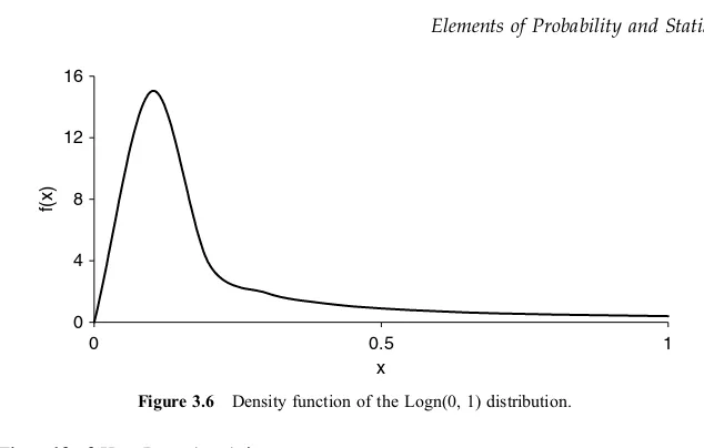
3.8.6 Lognormal Distribution 41 3.8.7 Gamma Distribution 42 3.8.8 Student´s t Distribution 44 3.8.9 F Distribution 45
3.8.10 Beta Distribution 46 3.8.11 Weibull Distribution 47
3.9 Stochastic Processes 47 3.9.1 Iid Processes 48 3.9.2 Poisson Processes 48
3.9.3 Regenerative (Renewal) Processes 49 3.9.4 Markov Processes 49
3.10 Estimation 50
3.11 Hypothesis Testing 51
Exercises 52
Chapter 4
Random Number and Variate Generation
4.1 Variate and Process Generation 56
4.2 Variate Generation Using the Inverse Transform Method 57 4.2.1 Generation of Uniform Variates 58
4.2.2 Generation of Exponential Variates 58 4.2.3 Generation of Discrete Variates 59
4.2.4 Generation of Step Variates from Histograms 60
4.3 Process Generation 61
4.3.1 Iid Process Generation 61 4.3.2 Non-Iid Process Generation 61
Exercises 63
Chapter 5
Arena Basics
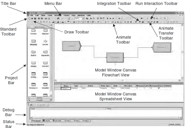
5.1 Arena Home Screen 66
5.1.1 MenuBar 67 5.1.2 ProjectBar 67 5.1.3 Standard Toolbar 68 5.1.4 Drawand ViewBars 68
5.1.7 IntegrationBar 69 5.1.8 DebugBar 69
5.2 Example: A Simple Workstation 69
5.3 Arena Data Storage Objects 74 5.3.1 Variables 75
5.3.2 Expressions 75 5.3.3 Attributes 75
5.4 Arena Output Statistics Collection 75
5.4.1 Statistics Collection via theStatisticModule 76 5.4.2 Statistics Collection via theRecord Module 76
5.5 Arena Simulation and Output Reports 77
5.6 Example: Two Processes in Series 78
5.7 Example: A Hospital Emergency Room 84 5.7.1 Problem Statement 84
5.7.2 Arena Model 85
5.7.3 Emergency Room Segment 86 5.7.4 On-Call Doctor Segment 93 5.7.5 Statistics Collection 96 5.7.6 Simulation Output 97
5.8 Specifying Time-Dependent Parameters via a
Schedule 100
Exercises 103
Chapter 6
Model Testing and Debugging Facilities
6.1 Facilities for Model Construction 107
6.2 Facilities for Model Checking 110
6.3 Facilities for Model Run Control 111 6.3.1 Run Modes 111
6.3.2 Mouse-Based Run Control 111 6.3.3 Keyboard-Based Run Control 112
6.4 Examples of Run Tracing 114
6.5 Visualization and Animation 118 6.5.1 Animate ConnectorsButton 118 6.5.2 Animate Toolbar 118
6.5.3 Animate TransferToolbar 119
6.6 Arena Help Facilities 119 6.6.1 HelpMenu 120 6.6.2 HelpButton 120
Exercises 120
Chapter 7
Input Analysis
7.1 Data Collection 124
7.2 Data Analysis 125
7.3 Modeling Time Series Data 127 7.3.1 Method of Moments 128
7.3.2 Maximal Likelihood Estimation Method 129
7.4 ArenaInput Analyzer 130
7.5 Goodness-of-Fit Tests for Distributions 134 7.5.1 Chi-Square Test 134
7.5.2 Kolmogorov-Smirnov (K-S) Test 137
7.6 Multimodal Distributions 137
Exercises 138
Chapter 8
Model Goodness: Verification and Validation
8.1 Model Verification via Inspection of Test Runs 142 8.1.1 Input Parameters and Output Statistics 142 8.1.2 Using a Debugger 143
8.1.3 Using Animation 143 8.1.4 Sanity Checks 143
8.2 Model Verification via Performance Analysis 143 8.2.1 Generic Workstation as a Queueing System 143 8.2.2 Queueing Processes and Parameters 144 8.2.3 Service Disciplines 145
8.2.5 Regenerative Queueing Systems and Busy Cycles 146 8.2.6 Throughput 147
8.2.7 Little´s Formula 148
8.2.8 Steady-State Flow Conservation 148 8.2.9 PASTA Property 149
8.3 Examples of Model Verification 149
8.3.1 Model Verification in a Single Workstation 149 8.3.2 Model Verification in Tandem Workstations 153
8.4 Model Validation 161
Exercises 162
Chapter 9
Output Analysis
9.1 Terminating and Steady-State Simulation Models 166 9.1.1 Terminating Simulation Models 166
9.1.2 Steady-State Simulation Models 166
9.2 Statistics Collection from Replications 168 9.2.1 Statistics Collection Using Independent
Replications 169
9.2.2 Statistics Collection Using Regeneration Points and Batch Means 170
9.3 Point Estimation 171
9.3.1 Point Estimation from Replications 171 9.3.2 Point Estimation in Arena 172
9.4 Confidence Interval Estimation 173
9.4.1 Confidence Intervals for Terminating Simulations 173 9.4.2 Confidence Intervals for Steady-State Simulations 176 9.4.3 Confidence Interval Estimation in Arena 176
9.5 Output Analysis via Standard Arena Output 177 9.5.1 Working Example: A Workstation with
Two Types of Parts 177 9.5.2 Observation Collection 179 9.5.3 Output Summary 180
9.5.4 Statistics Summary: Multiple Replications 181
9.6 Output Analysis via the ArenaOutput Analyzer 182 9.6.1 Data Collection 183
9.6.2 Graphical Statistics 184
9.6.4 Confidence Intervals for Means and Variances 186 9.6.5 Comparing Means and Variances 187
9.6.6 Point Estimates for Correlations 189
9.7 Parametric Analysis via the ArenaProcess Analyzer 190
Exercises 193
Chapter 10
Correlation Analysis
10.1 Correlation in Input Analysis 195
10.2 Correlation in Output Analysis 197
10.3 Autocorrelation Modeling with TES Processes 199
10.4 Introduction to TES Modeling 200 10.4.1 Background TES Processes 202 10.4.2 Foreground TES Processes 205 10.4.3 Inversion of Distribution Functions 211
10.5 Generation of TES Sequences 215 Generation of TESþSequences 215
Generation of TES Sequences 216
Combining TES Generation Algorithms 216
10.6 Example: Correlation Analysis in Manufacturing
Systems 219
Exercises 220
Chapter 11
Modeling Production Lines
11.1 Production Lines 223
11.2 Models of Production Lines 225
11.3 Example: A Packaging Line 225 11.3.1 An Arena Model 226
11.3.2 Manufacturing Process Modules 226
11.3.3 Model Blocking Using theHoldModule 227 11.3.4 Resources and Queues 229
11.4 Understanding System Behavior and Model Verification 237
11.5 Modeling Production Lines via Indexed Queues and
Resources 239
11.6 An Alternative Method of Modeling Blocking 246
11.7 Modeling Machine Failures 247
11.8 Estimating Distributions of Sojourn Times 251
11.9 Batch Processing 253
11.10 Assembly Operations 256
11.11 Model Verification for Production Lines 258
Exercises 259
Chapter 12
Modeling Supply Chain Systems
12.1 Example: A Production/Inventory System 265 12.1.1 Problem Statement 265
12.1.2 Arena Model 266
12.1.3 Inventory Management Segment 267 12.1.4 Demand Management Segment 270 12.1.5 Statistics Collection 272
12.1.6 Simulation Output 273
12.1.7 Experimentation and Analysis 274
12.2 Example: A Multiproduct Production/Inventory System 276 12.2.1 Problem Statement 276
12.2.2 Arena Model 278
12.2.3 Inventory Management Segment 278 12.2.4 Demand Management Segment 284 12.2.5 Model Input Parameters and Statistics 290 12.2.6 Simulation Results 292
12.3 Example: A Multiechelon Supply Chain 293 12.3.1 Problem Statement 293
12.3.2 Arena Model 295
12.3.3 Inventory Management Segment for Retailer 295 12.3.4 Inventory Management Segment
12.3.5 Inventory Management Segment for Output Buffer 299 12.3.6 Production/Inventory Management Segment
for Input Buffer 303
12.3.7 Inventory Management Segment for Supplier 305 12.3.8 Statistics Collection 305
12.3.9 Simulation Results 306
Exercises 306
Chapter 13
Modeling Transportation Systems
13.1 Advanced TransferTemplate Panel 314
13.2 Animate TransferToolbar 315
13.3 Example: A Bulk-Material Port 316 13.3.1 Ship Arrivals 317
13.3.2 Tug Boat Operations 320 13.3.3 Coal-Loading Operations 324 13.3.4 Tidal Window Modulation 328 13.3.5 Simulation Results 330
13.4 Example: A Toll Plaza 332 13.4.1 Arrivals Generation 334
13.4.2 Dispatching Cars to Tollbooths 336 13.4.3 Serving Cars at Tollbooths 340
13.4.4 Simulation Results for the Toll Plaza Model 344
13.5 Example: A Gear Manufacturing Job Shop 346 13.5.1 Gear Job Arrivals 349
13.5.2 Gear Transportation 351 13.5.3 Gear Processing 353
13.5.4 Simulation Results for the Gear Manufacturing Job Shop Model 358
13.6 Example: Sets Version of the Gear Manufacturing
Job Shop Model 359
Exercises 365
Chapter 14
Modeling Computer Information Systems
14.1.2 Client Hosts 372 14.1.3 Server Hosts 373
14.2 Communications Networks 374
14.3 Two-Tier Client/Server Example: A Human Resources
System 375
14.3.1 Client Nodes Segment 378
14.3.2 Communications Network Segment 378 14.3.3 Server Node Segment 380
14.3.4 Simulation Results 383
14.4 Three-Tier Client/Server Example: An Online Bookseller
System 384
14.4.1 Request Arrivals and Transmission Network Segment 386 14.4.2 Transmission Network Segment 388
A.1 Frequently Used Arena Built-in Variables 405 A.1.1 Entity-Related Attributes and Variables 405 A.1.2 Simulation Time Variables 406
A.1.9 Miscellaneous Variables and Functions 407
A.2 Frequently Used Arena Modules 407
A.2.11 HoldModule (Advanced Process) 410 A.2.12 MatchModule (Advanced Process) 410 A.2.13 PickStationModule (Advanced Transfer) 410 A.2.14 PickupModule (Advanced Process) 410 A.2.15 ProcessModule (Basic Process) 410 A.2.16 ReadWriteModule (Advanced Process) 411 A.2.17 RecordModule (Basic Process) 411 A.2.18 ReleaseModule (Advanced Process) 411 A.2.19 RemoveModule (Advanced Process) 411 A.2.20 RequestModule (Advanced Transfer) 411 A.2.21 RouteModule (Advanced Transfer) 412 A.2.22 SearchModule (Advanced Process) 412 A.2.23 SeizeModule (Advanced Process) 412 A.2.24 SeparateModule (Basic Process) 412 A.2.25 SignalModule (Advanced Process) 413 A.2.26 StationModule (Advanced Transfer) 413 A.2.27 StoreModule (Advanced Process) 413 A.2.28 TransportModule (Advanced Transfer) 413 A.2.29 UnstoreModule (Advanced Process) 413 A.2.30 VBABlock (Blocks) 414
Appendix B
VBA in Arena
B.1 Arena’s Object Model 416
B.2 Arena’s Type Library 416
B.2.1 Resolving Object Name Ambiguities 417 B.2.2 Obtaining Access to theApplication Object 417
B.3 Arena VBA Events 417
B.4 Example: Using VBA in Arena 419 B.4.1 Changing Inventory Parameters Just Before
a Simulation Run 419
B.4.2 Changing Inventory Parameters during a Simulation Run 421
B.4.3 Changing Customer Arrival Distributions Just before a Simulation Run 422
B.4.3 Writing Arena Data to Excel via VBA Code 424 B.4.4 Reading Arena Data from Excel via VBA Code 428
References
431
Preface
Monte Carlo simulation (simulation, for short) is a powerful tool for modeling and analysis of complex systems. The vast majority of real-life systems are difficult or impossible to study via analytical models due to the paucity or lack of practically computable solution (closed-form or numerical). In contrast, a simulation model can almost always be constructed and run to generate system histories that yield useful statistical information on system operation and performance measures. Simulation helps the analyst understand how well a system performs under a given regime or a set of parameters. It can also be used iteratively in optimization studies to find the best or acceptable values of parameters, mainly for offline design problems. Indeed, the scope of simulation is now extraordinarily broad, including manufacturing environments (semiconductor, pharmaceu-tical, among others), supply chains (production/inventory systems, distribution networks), transportation systems (highways, airports, railways, and seaports), computer information systems (client/server systems, telecommunications networks), and others. Simulation modeling is used extensively in industry as a decision-support tool in numerous industrial problems, including estimation of facility capacities, testing for alternative methods of operation, product mix decisions, and alternative system architectures. Almost every major engineering project in the past 30 years benefited from some type of simulation modeling and analysis. Some notable examples include the trans-Alaska natural gas pipeline project, the British channel tunnel (Chunnel) project, and operations scheduling for the Suez Canal. Simulation will doubtless continue to play a major role in performance analysis studies of complex systems for a long time to come.
Until the 1980s, simulation was quite costly and time consuming in terms of both analyst time and computing resources (memory and run time). The advent of inexpensive personal computers, with powerful processors and graphics, has ushered in new capabilities that rendered simulation a particularly attractive and cost-effective approach to performance analysis of a vast variety of systems. Simulation users can now construct and test simulation models interactively, and take advantage of extensive visualization and animation features. The programming of simulation models has been simplified in a paradigm that combines visual programming (charts) and textual programming (statements) and debugging capabilities (e.g., dynamic information display and animation of simulation objects). Finally, input and output analysis capabilities make it easier to model and analyze complex systems, while attractive output reports remove the tedium of programming simulation results.
Arena is a general-purpose visual simulation environment that has evolved over many years and many versions. It first appeared as the block-oriented SIMAN simulation language, and was later enhanced by the addition of many functional modules, full visualization of model structure and parameters, improved input and output analysis tools, run control and animation facilities, and output reporting. Arena has been widely used in both industry and academia; this book on simulation modeling and analysis uses Arena as the working simulation environment. A training version of Arena is enclosed with the book, and all book examples and exercises were designed to fit its vendor-imposed limitations.
This work is planned as a textbook for an undergraduate simulation course or a graduate simulation course at an introductory level. It aims to combine both theoretical and practical aspects of Monte Carlo simulation in general, as well as the workings of the Arena simulation environment. However, the book is not structured as a user manual for Arena, and we strongly recommend that readers consult the Arena help facilities for additional details on Arena constructs. Accordingly, the book is composed of four parts, as follows:
PART I
Chapters 1 to 4 lay the foundations by first reviewing system—theoretic aspects of simulation, followed by its probabilistic and statistical underpinnings, including random number generation.
Chapter 1 is an introduction to simulation describing the philosophy, trade-offs, and conceptual stages of the simulation modeling enterprise.
Chapter 2 reviews system theoretic concepts that underlie simulation, mainly discrete event simulation (DES) and the associated concepts of state, events, simulation clock, and event list. The random elements of simulation are introduced in a detailed example illustrating sample histories and statistics.
Chapter 3 is a compendium of information on the elements of probability, statistics, and stochastic processes that are relevant to simulation modeling.
Chapter 4 is a brief review of practical random number and random variate generation. It also briefly discusses generation of stochastic processes, such as Markov processes, but defers the discussion of generating more versatile autocorrelated stochastic sequences to the more advanced Chapter 10.
PART II
Chapters 5 and 6 introduce Arena basics and its facilities, and illustrate them in simple examples.
Chapter 6 is a brief review of the Arena testing and debugging facilities, including run control and interaction, as well as debugging, which are illustrated in detailed examples.
PART III
Chapters 7 to 10 address simulation-related theory (input analysis, validation, output analysis, and correlation analysis). They further illustrate concepts and their application using Arena examples of moderate complexity.
Chapter 7 treats input analysis (mainly distribution fitting) and the correspondingInput Analyzertool of Arena.
Chapter 8 discusses operational model verification via model inspection, and theory-based verification via performance analysis, using queueing theory (through-put, Little´s formula, and flow conservation principles). Model validation is also briefly discussed.
Chapter 9 treats output analysis (mainly replication design, estimation, and experimenta-tion for both terminating and steady-state simulaexperimenta-tions) and the corresponding ArenaOutput AnalyzerandProcess Analyzertools.
Chapter 10 introduces a new notion of correlation analysis that straddles input analysis and output analysis of autocorrelated stochastic processes. It discusses modeling and generation of autocorrelated sequences, and points out the negative consequences of ignoring temporal dependence in empirical data.
PART IV
Chapters 11 to 14 are applications oriented. They describe modeling of industrial applications in production, transportation, and information systems. These are illustrated in more elaborate Arena models that introduce advanced Arena constructs.
Chapter 11 addresses production lines, including finite buffers, machine failures, batch processing, and assembly operations.
Chapter 12 addresses supply chains, including production/inventory systems, multi-product systems, and multiechelon systems.
Chapter 13 addresses transportation systems, including tollbooth operations, port operations, and transportation activities on the manufacturing shop floor.
PART V
The book includes two appendices that provide Arena programming information.
Appendix A provides condensed information on frequently used Arena programming constructs.
Appendix B contains a condensed introduction to VBA (Visual Basic for Applications) programming in Arena.
Acknowledgments
We gratefully acknowledge the help of numerous individuals. We are indebted to Randy Sadowski, Rockwell Software, for supporting this effort. We thank our students and former students Baris Balcioglu, Pooya Farahvash, Cigdem Gurgur, Abdullah Karaman, Unsal Ozdogru, Mustafa Rawat, Ozgecan Uluscu, and Wei Xiong for their help and patience. We further thank Mesut Gunduc of Microsoft Corporation, Andrew T. Zador of ATZ Consultants, and Joe Pirozzi of Soros Associates for introducing us to a world of challenging problems in computer information systems and transportation systems. We also thank Dr. David L. Jagerman for his longtime collaboration on mathematical issues, and the National Science Foundation for support in the areas of performance analysis of manufacturing and transportation systems, and correlation analysis.
Last but not least we are grateful to our respective spouses, Binnur Altiok and Shulamit Melamed, for their support and understanding of our hectic schedule in the course of writing this book.
Tayfur Altiok Benjamin Melamed June 2007
Introduction to
Simulation Modeling
Simulation modeling is a common paradigm for analyzing complex systems. In a nutshell, this paradigm creates a simplified representation of a system under study. The paradigm then proceeds to experiment with the system, guided by a prescribed set of goals, such as improved system design, cost–benefit analysis, sensitivity to design parameters, and so on. Experimentation consists of generating system histories and observing system behavior over time, as well as its statistics. Thus, the representation created (see Section 1.1) describes system structure, while the histories generated describe system behavior (see Section 1.5).
This book is concerned with simulation modeling of industrial systems. Included are manufacturing systems (e.g., production lines, inventory systems, job shops, etc.), supply chains, computer and communications systems (e.g., client-server systems, communi-cations networks, etc.), and transportation systems (e.g., seaports, airports, etc.). The book addresses both theoretical topics and practical ones related to simulation modeling. Throughout the book, the Arena/SIMAN (see Keltonet al. 2000) simulation tool will be surveyed and used in hands-on examples of simulation modeling.
This chapter overviews the elements of simulation modeling and introduces basic concepts germane to such modeling.
1.1
SYSTEMS AND MODELS
Modeling is the enterprise of devising a simplified representation of a complex system with the goal of providing predictions of the system's performance measures (metrics) of interest. Such a simplified representation is called a model. A model is designed to capture certain behavioral aspects of the modeled system—those that are of interest to the analyst/modeler—in order to gain knowledge and insight into the system's behavior (Morris 1967).
Modeling calls for abstraction and simplification. In fact, if every facet of the system under study were to be reproduced in minute detail, then the model cost may approach that of the modeled system, thereby militating against creating a model in the first place.
Simulation Modeling and Analysis with Arena
The modeler would simply use the “real” system or build an experimental one if it does not yet exist—an expensive and tedious proposition. Models are typically built precisely to avoid this unpalatable option. More specifically, while modeling is ultim-ately motivated by economic considerations, several motivational strands may be discerned:
Evaluating system performance under ordinary and unusual scenarios. A model may be a necessity if the routine operation of the real-life system under study cannot be disrupted without severe consequences (e.g., attempting an upgrade of a production line in the midst of filling customer orders with tight deadlines). In other cases, the extreme scenario modeled is to be avoided at all costs (e.g., think of modeling a crash-avoiding maneuver of manned aircraft, or core meltdown in a nuclear reactor).
Predicting the performance of experimental system designs. When the underlying system does not yet exist, model construction (and manipulation) is far cheaper (and safer) than building the real-life system or even its prototype. Horror stories appear periodically in the media on projects that were rushed to the implementation phase, without proper verification that their design is adequate, only to discover that the system was flawed to one degree or another (recall the case of the brand new airport with faulty luggage transport).
Ranking multiple designs and analyzing their tradeoffs. This case is related to the previous one, except that the economic motivation is even greater. It often arises when the requisition of an expensive system (with detailed specifications) is awarded to the bidder with the best cost–benefit metrics.
Models can assume a variety of forms:
Aphysical modelis a simplified or scaled-down physical object (e.g., scale model of an airplane).
Amathematicaloranalytical modelis a set of equations or relations among mathemat-ical variables (e.g., a set of equations describing the workflow on a factory floor).
Acomputer modelis just a program description of the system. A computer model with random elements and an underlying timeline is called aMonte Carlo simulation model (e.g., the operation of a manufacturing process over a period of time).
Monte Carlo simulation, orsimulationfor short, is the subject matter of this book. We shall be primarily concerned with simulation models of production, transportation, and computer information systems. Examples include production lines, inventory systems, tollbooths, port operations, and database systems.
1.2
ANALYTICAL VERSUS SIMULATION MODELING
A simulation model is implemented in a computer program. It is generally a relatively inexpensive modeling approach, commonly used as an alternative to analytical model-ing. The tradeoff between analytical and simulation modeling lies in the nature of their
“solutions,”that is, the computation of their performance measures as follows:
2. A simulation model calls for running (executing) a simulation program to produce sample histories. A set of statisticscomputed from these histories is then used to form performance measures of interest.
To compare and contrast both approaches, suppose that a production line is concep-tually modeled as a queuing system. The analytical approach would create an analytical queuing system (represented by a set of equations) and proceed to solve them. The simulation approach would create a computer representation of the queuing system and run it to produce a sufficient number of sample histories. Performance measures, such as average work in the system, distribution of waiting times, and so on, would be constructed from the corresponding“solutions”as mathematical or simulation statistics, respectively.
The choice of an analytical approach versus simulation is governed by general tradeoffs. For instance, an analytical model ispreferableto a simulation model when it has a solution, since its computation is normally much faster than that of its simula-tion-model counterpart. Unfortunately, complex systems rarely lend themselves to modeling via sufficiently detailed analytical models. Occasionally, though rarely, the numerical computation of an analytical solution is actually slower than a corresponding simulation. In the majority of cases, an analytical model with a tractable solution is unknown, and the modeler resorts to simulation.
When the underlying system is complex, a simulation model is normallypreferable, for several reasons. First, in the unlikely event that an analytical model can be found, the modeler's time spent in deriving a solution may be excessive. Second, the modeler may judge that an attempt at an analytical solution is a poor bet, due to the apparent mathematical difficulties. Finally, the modeler may not even be able to formulate an analytical model with sufficient power to capture the system's behavioral aspects of interest. In contrast, simulation modeling can capture virtually any system, subject to any set of assumptions. It also enjoys the advantage of dispensing with the labor attendant to finding analytical solutions, since the modeler merely needs to construct and run a simulation program. Occasionally, however, the effort involved in construct-ing an elaborate simulation model is prohibitive in terms of human effort, or runnconstruct-ing the resultant program is prohibitive in terms of computer resources (CPU time and memory). In such cases, the modeler must settle for a simpler simulation model, or even an inferior analytical model.
Another way to contrast analytical and simulation models is via the classification of models intodescriptiveorprescriptive models. Descriptive models produce estimates for a set of performance measures corresponding to a specific set of input data. Simulation models are clearly descriptive and in this sense serve as performance analysis models. Prescriptive models are naturally geared toward design or optimization (seeking the optimal argument values of a prescribed objective function, subject to a set of constraints). Analytical models are prescriptive, whereas simulation is not. More specifically, analytical methods can serve as effective optimization tools, whereas simulation-based optimization usually calls for an exhaustive search for the optimum.
In particular, the complexity of industrial and service systems often forces the issue of selecting simulation as the modeling methodology of choice.
1.3
SIMULATION MODELING AND ANALYSIS
The advent of computers has greatly extended the applicability of practical simula-tion modeling. Since World War II, simulasimula-tion has become an indispensable tool in many system-related activities. Simulation modeling has been applied to estimate performance metrics, to answer“what if”questions, and more recently, to train workers in the use of new systems. Examples follow.
Estimating a set of productivity measures in production systems, inventory systems, manufacturing processes, materials handling, and logistics operations
Designing and planning the capacity of computer systems and communication networks so as to minimize response times
Conducting war games to train military personnel or to evaluate the efficacy of proposed military operations
Evaluating and improving maritime port operations, such as container ports or bulk-material marine terminals (coal, oil, or minerals), aimed at finding ways of reducing vessel port times
Improving health care operations, financial and banking operations, and transportation systems and airports, among many others
In addition, simulation is now used by a variety of technology workers, ranging from design engineers to plant operators and project managers. In particular, manufac-turing-related activities as well as business process reengineering activities employ simulation to select design parameters, plan factory floor layout and equipment pur-chases, and even evaluate financial costs and return on investment (e.g., retooling, new installations, new products, and capital investment projects).
1.4
SIMULATION WORLDVIEWS
Aworldviewis a philosophy or paradigm. Every computer tool has two associated worldviews: a developer worldview and a user worldview. These two worldviews should be carefully distinguished. The first worldview pertains to the philosophy adopted by the creators of the simulation software tool (in our case, software designers and engineers). The second worldview pertains to the way the system is employed as a tool by end-users (in our case, analysts who create simulation models as code written in somesimulation language). A system worldview may or may not coincide with an end-user worldview, but the latter includes the former.
simulation event occurs, at which point the model undergoes a state transition. The model evolution is governed by aclockand a chronologically orderedevent list. Each event is implemented as a procedure (computer code) whose execution can change state variables and possibly schedule other events. A simulation run is started by placing an initial event in the event list, proceeds as an infinite loop that executes the current most imminent event (the one at the head of the event list), and ends when an event stops or the event list becomes empty. This beguilingly simple paradigm is extremely general and astonishingly versatile.
Early simulation languages employed a user worldview that coincided with the discrete-event paradigm. A more convenient, but more specialized, paradigm is the transaction-driven paradigm (commonly referred to as process orientation). In this popular paradigm, there are two kinds of entities:transactions and resources. A resource is a service-providing entity, typically stationary in space (e.g., a machine on the factory floor). A transaction is a mobile entity that moves among“geographical”
locations (nodes). A transaction may experience delays while waiting for a resource due to contention (e.g., a product that moves among machines in the course of assem-bly). Transactions typically go through a life cycle: they get created, spend time at various locations, contend for resources, and eventually depart from the system. The computer code describing a transaction's life cycle is called aprocess.
Queuing elements figure prominently in this paradigm, since facilities typically contain resources and queues. Accordingly, performance measures of interest include statistics of delays in queues, the number of transactions in queues, utilization, uptimes and downtimes of resources subject to failure, and lost demand, among many others.
1.5
MODEL BUILDING
Modeling, including simulation modeling, is a complicated activity that combines art and science. Nevertheless, from a high-level standpoint, one can distinguish the following major steps:
1. Problem analysis and information collection. The first step in building a simula-tion model is to analyze the problem itself. Note that system modeling is rarely undertaken for its own sake. Rather, modeling is prompted by some system-oriented problem whose solution is the mission of the underlying project. In order to facilitate a solution, the analyst first gathers structural information that bears on the problem, and represents it conveniently. This activity includes the identifi-cation of input parameters, performance measures of interest, relationships among parameters and variables, rules governing the operation of system components, and so on. The information is then represented as logic flow diagrams, hierarchy trees, narrative, or any other convenient means of representation. Once sufficient information on the underlying system is gathered, the problem can be analyzed and a solution mapped out.
model validation. That is, data collected on system output statistics are compared to their model counterparts (predictions).
3. Model construction. Once the problem is fully studied and the requisite data collected, the analyst can proceed to construct a model and implement it as a computer program. The computer language employed may be a general-purpose language (e.g., C++, Visual Basic, FORTRAN) or a special-purpose simulation language or environment (e.g., Arena, Promodel, GPSS). See Section 2.4 for details.
4. Model verification. The purpose of model verification is to make sure that the model is correctly constructed. Differently stated, verification makes sure that the model conforms to its specification and does what it is supposed to do. Model verification is conducted largely by inspection, and consists of comparing model code to model specification. Any discrepancies found are reconciled by modifying either the code or the specification.
5. Model validation. Every model should be initially viewed as a mere proposal, subject to validation. Model validation examines the fit of the model to empirical data (measurements of the real-life system to be modeled). A good model fit means here that a set of important performance measures, predicted by the model, match or agree reasonably with their observed counterparts in the real-life system. Of course, this kind of validation is only possible if the real-life system or emulation thereof exists, and if the requisite measurements can actually be acquired. Any significant discrepancies would suggest that the proposed model is inadequate for project purposes, and that modifications are called for. In practice, it is common to go through multiple cycles of model construction, verification, validation, and modification.
6. Designing and conducting simulation experiments. Once the analyst judges a model to be valid, he or she may proceed to design a set of simulation experiments (runs) to estimate model performance and aid in solving the project's problem (often the problem is making system design decisions). The analyst selects a number of scenarios and runs the simulation to glean insights into its workings. To attain sufficient statistical reliability of scenario-related performance measures, each scenario is replicated (run multiple times, subject to different sequences of random numbers), and the results averaged to reduce statistical variability. 7. Output analysis. The estimated performance measures are subjected to a thorough
logical and statistical analysis. A typical problem is one of identifying the best design among a number of competing alternatives. A statistical analysis would run statistical inference tests to determine whether one of the alternative designs enjoys superior performance measures, and so should be selected as the apparent best design.
8. Final recommendations. Finally, the analyst uses the output analysis to formulate the final recommendations for the underlying systems problem. This is usually part of a written report.
1.6
SIMULATION COSTS AND RISKS
Modeling cost. Like any other modeling paradigm, good simulation modeling is a prerequisite to efficacious solutions. However, modeling is frequently more art than science, and the acquisition of good modeling skills requires a great deal of practice and experience. Consequently, simulation modeling can be a lengthy and costly process. This cost element is, however, a facet of any type of modeling. As in any modeling enterprise, the analyst runs the risk of postulating an inaccurate or patently wrong model, whose invalidity failed to manifest itself at the validation stage. Another pitfall is a model that incorporates excessive detail. The right level of detail depends on the underlying problem. The art of modeling involves the construction of the least-detailed model that can do the job (producing adequate answers to questions of interest).
Coding cost. Simulation modeling requires writing software. This activity can be error-prone and costly in terms of time and human labor (complex software projects are notorious for frequently failing to complete on time and within budget). In addition, the ever-present danger of incorrect coding calls for meticulous and costly verification.
Simulation runs. Simulation modeling makes extensive use of statistics. The analyst should be careful to design the simulation experiments, so as to achieve adequate statistical reliability. This means that both the number of simulation runs (replications) and their length should be of adequate magnitude. Failing to do so is to risk the statistical reliability of the estimated performance measures. On the other hand, some simulation models may require enormous computing resources (memory space and CPU time). The modeler should be careful not to come up with a simulation model that requires prohibi-tive computing resources (clever modeling and clever code writing can help here).
Output analysis. Simulation output must be analyzed and properly interpreted. Incor-rect predictions, based on faulty statistical analysis, and improper understanding of system behavior are ever-present risks.
1.7
EXAMPLE: A PRODUCTION CONTROL PROBLEM
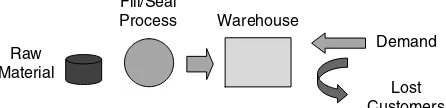
This section presents a simple production control problem as an example of the kind of systems amenable to simulation modeling. This example illustrates system definition and associated performance issues. A variant of this system will be discussed in Section 11.3, and its Arena model will be presented there.
Consider a packaging/warehousing process with the following steps:
1. The product is filled and sealed.
2. Sealed units are placed into boxes and stickers are placed on the boxes. 3. Boxes are transported to the warehouse to fulfill customer demand.
These steps can be combined into a single processing time, as depicted in the system schematic of Figure 1.1.
The system depicted in Figure 1.1 is subject to the following assumptions:
1. There is always sufficient raw material for the process never tostarve.
2. Processing is carried out in batches, five units to a batch. Finished units are placed in the warehouse. Data collected indicate that unit-processing times are uniformly distributed between 10 and 20 minutes.
3. The process experiencesrandom failures, which may occur at any point in time. Times between failures are exponentially distributed with a mean of 200 minutes. Data collection also showed that repair times are normally distributed, with a mean of 90 minutes and a standard deviation of 45 minutes.
4. The warehouse has a capacity(target level) ofR¼500 units. Processing stops when the inventory in the warehouse reaches the target level. From this point on, the production process becomesblockedand remains inactive until the inventory level drops to the reorder point, which is assumed to be r¼150 units. The process restarts with a new batch as soon as the reorder level is down-crossed. This is a convenient policy when a resource needs to be distributed among various types of products. For instance, when our process becomes blocked, it may actually be assigned to another task or product that is not part of our model. 5. Data collection shows that interarrival times between successive customers are
uniformly distributed between 3 and 7 hours, and that individual demand sizes are distributed uniformly between 50 and 100 units. On customer arrival, the inventory is immediately checked. If there is sufficient stock on hand, that demand is promptly satisfied; otherwise, customer demand is either partially satisfied and the rest is lost (that is, the unsatisfied portion represents lost business), or the entire demand is lost, depending on the availability of finished units and the loss policy employed.
This problem is also known as aproduction/inventory problem. We mention, how-ever, that the present example is a gross simplification. More realistic production/ inventory problems have additional wrinkles, including multiple types of products, production setups or startups, and so on. Some design and performance issues and associated performance measures of interest follow:
1. Can we improve the customer service level (percentage of customers whose demand is completely satisfied)?
2. Is the machinery underutilized or overutilized (machine utilization)? 3. Is the maintenance level adequate (downtime probabilities)?
4. What is the tradeoff between inventory level and customer service level?
The previous list is far from being exhaustive, and the actual requisite list will, of course, depend on the problem to be solved.
1.8
PROJECT REPORT
A project report should be clearly and plainly written, so that nontechnical people as well as professionals can understand it. This is particularly true for project conclusions and recommendations, as these are likely to be read by management as part of the decision-making process. Although one can hardly overemphasize the importance of project reporting, the topic of proper reporting is rarely addressed explicitly in the published literature. In practice, analysts learn project-writing skills on the job, typically by example.
A generic simulation project report addresses the model building stages described in Section 1.5, and consists of (at least) the following sections:
Cover page. Includes a project title, author names, date, and contact information in this order. Be sure to compose a descriptive but pithy project title.
Executive summary. Provides a summary of the problem studied, model findings, and conclusions.
Table of contents. Lists section headings, figures, and tables with the corresponding page numbers.
Introduction. Sets up the scene with background information on the system under study (if any), the objectives of the project, and the problems to be solved. If appropriate, include a brief review of the relevant company, its location, and products and services.
System description. Describes in detail the system to be studied, using prose, charts, and tables (see Section 1.7). Include all relevant details but no more (the rest of the book and especially Chapters 11–13 contain numerous examples).
Input analysis. Describes empirical data collection and statistical data fitting (see Section 1.5 and Chapter 7). For example, the Arena Input Analyzer (Section 7.4) provides facilities for fitting distributions to empirical data and statistical tests. More advanced model fitting of stochastic processes to empirical data is described in Chapter 10.
Simulation model description. Describes the modeling approach of the simulation model, and outlines its structure in terms of its main components, objects, and the operational logic. Be sure to decompose the description of a complex model into manageable-size submodel descriptions. Critical parts of the model should be described in some detail.
Verification and validation. Provides supportive evidence for model goodness via model verification and validation (see Section 1.5) to justify its use in predicting the performance measures of the system under study (see Chapter 8). To this end, be sure to address at least the following two issues: (1) Does the model appear to run correctly and to provide the relevant statistics (verification)? (2) If the modeled system exists, how close are its statistics (e.g., mean waiting times, utilizations, throughputs, etc.) to the corresponding model estimates (validation)?
Output analysis. Describes simulation model outputs, including run scenarios, number of replications, and the statistical analysis of simulation-produced observations (see Chapter 9). For example, the Arena Output Analyzer (Section 9.6) provides facilities for data graphing, statistical estimation, and statistical comparisons, while the Arena Process Analyzer (Section 9.7) facilitates parametric analysis of simulation models.
Simulation results. Collects and displays summary statistics of multiple replicated scenarios. Arena's report facilities provide the requisite summary statistics (numerous reports are displayed in the sequel).
that produce improvements, such as better performance and reduced costs. Be sure to discuss thoroughly the impact of suggested modifications by quantifying improvements and analyzing tradeoffs where relevant.
Conclusions and recommendations. Summarizes study findings and furnishes a set of recommendations.
Appendices. Contains any relevant material that might provide undesired digression in the report body.
Needless to say, the modeler/analyst should not hesitate to customize and modify the previous outlined skeleton as necessary.
EXERCISES
1. Consider an online registration system (e.g., course registration at a university or membership registration in a conference).
a. List the main components of the system and its transactions.
b. How would you define the state and events of each component of the registra-tion system?
c. Which performance measures might be of interest to registrants?
d. Which performance measures might be of interest to the system administrator? e. What data would you collect?
2. The First New Brunswick Savings (FNBS) bank has a branch office with a number of tellers serving customers in the lobby, a teller serving the drive-in line, and a number of service managers serving customers with special requests. The lobby, drive-in, and service managers each have a separate single queue. Customers may join either of the queues (the lobby queue, the drive-in queue, or the service managers’ queue). FNBS is interested in performance evaluation of their customer service operations.
a. What are the random components in the system and their parameters? b. What performance measures would you recommend FNBS to consider? c. What data would you collect and why?
3. Consider the production/inventory system of Section 1.7. Suppose the system produces and stores multiple products.
a. List the main components of the system and its transactions as depicted in Figure 1.1.
b. What are the transactions and events of the system, in view of Figure 1.1? c. Which performance measures might be of interest to customers, and which to
owners?
Discrete Event Simulation
The majority of modern computer simulation tools (simulators) implement a para-digm, calleddiscrete-event simulation(DES). This paradigm is so general and powerful that it provides an implementation framework for most simulation languages, regardless of the user worldview supported by them. Because this paradigm is so pervasive, we will review and explain in this chapter its working in some detail.
2.1
ELEMENTS OF DISCRETE EVENT SIMULATION
In the DES paradigm, the simulation model possesses a state S (possibly vector-valued) at any point in time. A system state is a set of data that captures the salient variables of the system and allows us to describe system evolution over time. In a computer simulation program, the state is stored in one or more program variables that represent various data structures (e.g., the number of customers in a queue, or their exact sequence in the queue). Thus, the state can be defined in various ways, depending on particular modeling needs, and the requisite level of detail is incorporated into the model. As an example, consider a machine, fed by a raw-material storage of jobs. A“coarse”state of the system is the number jobs in the storage; note, however, that this state definition does not permit the computation of waiting times, because the identity of individual jobs is not maintained. On the other hand, the more“refined”state consisting of customer identities in a queue and associated data (such as customer arrival times) does permit the computation of waiting times. In practice, the state definition of a system should be determined based on its modeling needs, particularly the statistics to be computed.
The state trajectory over time, S(t), is abstracted as a step function, whose jumps (discontinuities) are triggered by discreteevents, which inducestate transactions(changes in the system state) at particular points in time. Although computer implementation of events varies among DES simulators, they are all conceptually similar: An event is a data structure that always has a field containing its time of occurrence, and any number of other fields. Furthermore, the“occurrence”of an event in a DES simulator is implemented as the execution of a corresponding procedure (computer code) at the scheduled event occur-rence time. When that procedure is run, we say that the event isprocessedorexecuted.
Simulation Modeling and Analysis with Arena
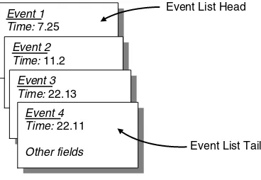
The evolution of any DES model is governed by a clock and a chronologically orderedevent list. That is, events are linked in the event list according to their scheduled order of occurrence (Figure 2.1). The event at the head of the list is called the most imminent eventfor obvious reasons.Scheduling an eventmeans that the event is linked chronologically into the event list. Theoccurrenceof an event means that the event is unlinked from the event list and executed. The execution of an event can change state variables and possibly schedule other events in the event list.
An essential feature of the DES paradigm is that“nothing”changes the state unless an event occurs, at which point the model typically undergoes a state transition. More precisely, every event execution can change the state (although on rare occasions the state remains intact), but every state change is effected by some event. Between events, the state of the DES is considered constant, even though the system is engaged in some activity. For example, consider a machine on the factory floor that packages beer cans into six-packs, such that the next six-pack is loaded for processing only when the previous one has been completely processed. Suppose that the state tracks the number of six-packs waiting to be processed at any given time. Then during the processing time of a six-pack, the DES state remains unchanged, even though the machine may, in fact, be processing six beer cans individually. The DES state will only be updated when the entire six-pack is processed; this state change will be triggered by a“six-pack comple-tion”event. Note again that the definition of the state is up to the modeler, and that models can be refined by adding new types of events that introduce additional types of state transitions.
At the highest level of generalization, a DES simulator executes the following algorithm:
1. Set the simulation clock to an initial time (usually 0), and then generate one or more initial events and schedule them.
2. If the event list is empty, terminate the simulation run. Otherwise, find the most imminent event and unlink it from the event list.
3. Advance the simulation clock to the time of the most imminent event, and execute it (the event may stop the simulation).
4. Loop back to Step 2.
This beguilingly simple algorithm (essentially an infinite loop) is extremely general. Its complexity is hidden in the routines that implement event execution and the data structures used by them. The power and versatility of the DES simulation algorithm
Event 1
stem from the fact that the DES paradigm naturally scales to collections of interacting subsystems: one can build hierarchies of increasingly complex systems from subsystem components. In addition, the processing of any event can be as intricate as desired. Thus, both large systems as well as complex ones can be represented in the DES paradigm. (For more details, see Fishman 1973, Banks et al. 1999, and Law and Kelton 2000.)
2.2
EXAMPLES OF DES MODELS
In this section the power and generality of DES models are illustrated through several examples of elementary systems. The examples illustrate how progressively complex DES models can be constructed from simpler ones, either by introducing new modeling wrinkles that increase component complexity, or by adding components to create larger DES models.
2
.
2
.
1
S
INGLEM
ACHINEConsider a failure-proof single machine on the shop floor, fed by a buffer. Arriving jobs that find the machine busy (processing another job) must await their turn in the buffer, and eventually are processed in their order of arrival. Such a service discipline is called FIFO (first in first out) or FCFS (first come first served), and the resulting system is called a queue or queueing system. (The word“queue”is derived from French and ultimately from a Latin word that means“tail,”which explains its technical meaning as a“waiting line.”Its quaint spelling renders it one of the most vowel-redundant words in the English language.) Suppose that job interarrival times and processing times are given (possibly random). A schematic description of the system is depicted in Figure 2.2. To represent this system as a DES, define the stateS(t) to be the number of jobs in the system at timet. Thus,S(t)¼5 means that at timet, the machine is busy processing the first job and 4 more jobs are waiting in the buffer. There are two types of events: arrivalsand process completions. Suppose that an arrival took place at time t, when there wereS(t)¼njobs in the system. Then the value ofS jumps at timetfromnto nþ1, and this transition is denoted by n!nþ1. Similarly, a process completion is described by the transition n!n 1. Both transitions are implemented in the simulation program as part of the corresponding event processing.
2
.
2
.
2
S
INGLEM
ACHINE WITHF
AILURESConsider the previous single machine on the shop floor, now subject to failures. In addition to arrival and service processes, we now also need to describe times to
Job
failure as well as repair times. We assume that the machine fails only while processing a job, and that on repair completion, the job has to be reprocessed from scratch. A schematic description of the system is depicted in Figure 2.3.
The stateS(t) is a pair of variables,S(t)¼(N(t), V(t) ), whereN(t) is the number of jobs in the buffer, andV(t) is the process status (idle, busy, or down), all at timet. In a simulation program,V(t) is coded, say by integers, as follows: 0¼idle, 1¼busy, and 2¼ down. Note that one job must reside at the machine, whenever its status isbusyordown. The events arearrivals,process completions,machine failures, andmachine repairs. The corresponding state transitions follow:
Consider the single machine on a shop floor, without failures. Jobs that finish processing go to an inspection station with its own buffer, where finished jobs are checked for defects. Jobs that pass inspection are stored in a finished inventory ware-house. However, jobs that fail inspection are routed back to the tail end of the machine's buffer for reprocessing. In addition to interarrival times and processing times, we need here a description of the inspection time as well as the inspection decision (pass/fail) mechanism (e.g., jobs fail with some probability, independently of each other). A schematic description of the system is depicted in Figure 2.4.
The state S(t) is a triplet of variables, S(t)¼(N(t), I(t), K(t) ) where N(t) is the number of items in the machine and its buffer, I(t) is the number of items at the inspection station, and K(t) is the storage content, all at time t. Events consist of arrivals, process completions, inspection failure (followed by routing to the tail end of the machine's buffer), andinspection passing(followed by storage in the warehouse). The corresponding state transitions follow:
Job arrival: (n, i, k)!(nþ1, i, k)
Process completion: (n, i, k)!(n 1, iþ1, k)
Inspection completion: (n, i, k)! (n(n,þi1,i1,k1,k), if job failed inspection þ1), if job passed inspection
2.3
MONTE CARLO SAMPLING AND HISTORIES
Monte Carlo simulation models incorporate randomness by sampling random values from specified distributions. The underlying algorithms and/or their code userandom number generators(RNG) that produce uniformly distributed values (“equally likely”) between 0 and 1; these values are then transformed to conform to a prescribed dis-tribution. We add parenthetically that the full term ispseudo RNGto indicate that the numbers generated are not“truly”random (they can be reproduced algorithmically), but only random in a statistical sense; however, the prefix“pseudo”is routinely dropped for brevity. This general sampling procedure is referred to as Monte Carlo sampling. The name is attributed to von Neumann and Ulam for their work at Los Alamos National Laboratory (see Hammersly and Handscomb 1964), probably as an allusion to the famous casino at Monte Carlo and the relation between random number generation and casino gambling.
In particular, the random values sampled using RNGs are used (among other things) to schedule events at random times. For the most part, actual event times are determined by sampling an interevent time (e.g., interarrival times, times to failure, repair times, etc.) via an RNG, and then adding that value to the current clock time. More details are presented in Chapter 4.
DES runs use a statistical approach to evaluating system performance; in fact, simulation-based performance evaluation can be thought of as a statistical experiment. Accordingly, the requisite performance measures of the model under study are not computed exactly, but rather, they are estimated from a set of histories. A standard statistical procedure unfolds as follows:
1. The modeler performs multiple simulation runs of the model under study, using independent sequences of random numbers. Each run is called areplication. 2. One or more performance measures are computed from each replication. Examples
include average waiting times in a queue, average WIP (work in process) levels, and downtime probabilities.
3. The performance values obtained are actually random and mutually independent, and together form a statistical sample. To obtain a more reliable estimate of the true value of each performance metric, the corresponding values are averaged and confidence intervals about them are constructed. This is discussed in Chapter 3.
Warehouse
2
.
3
.
1
E
XAMPLE: W
ORKS
TATIONS
UBJECT TOF
AILURES ANDI
NVENTORYC
ONTROLThis section presents a detailed example that illustrates the random nature of DES modeling and simulation runs, including the random state and its sample paths. Our goal is to study system behavior and estimate performance metrics of interest. To this end, consider the workstation depicted in Figure 2.5.
The system is comprised of a machine, which never starves (always has a job to work on), and a warehouse that stores finished products (jobs). In addition, the machine is subject to failures, and its status is maintained in the random variableV(t), given by
V(t)¼
Note that one job must reside at the machine, whenever its status is busy or down. The stateS(t) is a pair of variables,S(t)¼(V(t),K(t)) whereV(t) is the status of the machine as described previously, andK(t) is the finished-product level in the warehouse, all at timet. For example, the stateS(t)¼(2, 3) indicates that at timetthe machine is down (presumably being repaired), and the warehouse has an inventory of three finished product units. Customer orders (demand) arrive at the warehouse, and filled orders deplete the inventory by the ordered amount (orders that exceed the stock on hand are partially filled, the shortage simply goes unfilled, and no backorder is issued). The product unit processing time is 10 minutes. In this example, the machine does not operate independently, but rather is controlled by the warehouse as follows. Whenever the inven-tory level reaches or drops belowr¼2 units (called thereorder point), the warehouse issues a replenishment request to the machine to bring the inventory up to the level ofR¼ 5 units (calledtarget levelorbase-stock level). In this case, the inventory level is said to down-cross the reorder point. At this point, the machine starts processing a sequence of jobs until the inventory level reaches the target value, R, at which point the machine suspends operation. Such a control regime is known as the (r,R) continuous reviewinventory control policy (or simply as the (r,R) policy), and the corresponding replenishment regime is referred to as apull system. See Chapter 12 for detailed examples.
Sample History
Suppose that events occur in the DES model of the workstation above in the order shown in Figure 2.6, which graphs the stock on hand in the warehouse as a function of
Demand
time, and also tracks the status of the machine,V(t), over time. (Note that Figure 2.6 depicts a sample history—one of many possible histories that may be generated by the simulated system.)
An examination of Figure 2.6 reveals that at timet¼0, the machine is idle and the warehouse contains four finished units, that is, V(0) ¼ 0 and K(0) ¼ 4. The first customer arrives at the warehouse at timet¼35 and demands three units. Since the stock on hand can satisfy this order, it is depleted by three units, resulting inK(35)¼1; at this point, the reorder point,r, is down-crossed, triggering a replenishment request at the machine that resumes the production of additional product in order to raise the inventory level to its target value,R. Note that the machine status changes concomi-tantly fromidletobusy. During the next 30 minutes, no further demand arrives, and the inventory level climbs gradually as finished products arrive from the machine, until reaching a level of 4 at timet¼65.
At time t ¼ 69, a second customer arrives and places a demand equal or larger than the stock on hand, thereby depleting the entire inventory. Since unsatisfied demand goes unfilled, we haveK(69)¼ 0. If backorders were allowed, then we would keep track of the backorder size represented by the magnitude of the corresponding negative inventory.
At time t ¼75, the unit that started processing at the machine at time t ¼65 is finished and proceeds to the warehouse, so thatK(75)¼1. Another unit is finished with processing at the machine at timet¼85.
At time t ¼ 87, the machine fails and its repair begins (down state). The repair activity is completed at timet¼119 and the machine status changes tobusy. While the machine is down, a customer arrives at time t ¼ 101, and the associated demand decreases the stock on hand by one unit, so thatK(101) ¼ 1. At time t¼ 119, the repaired machine resumes processing of the unit whose processing was interrupted at the time of failure; that unit completes processing at timet¼127.
From time t ¼ 127 to time t ¼ 157 no customers arrive at the warehouse, and consequently the inventory reaches its target level,R ¼5, at timet¼157, at which time the machine suspends production. The simulation run finally terminates at time T¼165.
Sample Statistics
Having generated a sample history of system operation, we can now proceed to compute associated statistics (performance measures).
Probability distribution of machine status. Consider the machine status over the time interval [0,T]. LetTI be the total idle time over [0,T],TBthe total busy time over [0,T],
andTD the total downtime over [0,T]. The probability distribution of machine status
is then estimated by the ratios of time spent in a state to total simulation time, namely,
Pr{machine idle}¼TI
In particular, the probability that the machine is busy coincides with the server utiliza-tion (the fracutiliza-tion of time the machine is actually busy producing). Note that all the probabilities above are estimated bytime averages, which here assume the form of the fraction of time spent by the machine in each state (the general form of time averages is discussed in Section 9.3). The logic underlying these definitions is simple. If an outside observer“looks”at the system at random, then the probability of finding the machine in a given state isproportionalto the total time spent by the machine in that state. Of course, the ratios (proportions) above sum to unity, by definition.
Machine throughput. Consider the number of job completionsCT in the machine
over the interval [0, T]. The throughput is a measure of effective processing rate, namely, the expected number of job completions (and, therefore, departures) per unit time, estimated by
Customer service level. Consider customers arriving at the warehouse with a demand for products. LetNS be the number of customers whose demand is fully satisfied over
the interval [0,T], andNT the total number of customers that arrived over [0,T]. The
customer service level,x, is the probability of fully satisfying the demand of an arrival at the warehouse. This performance measure is estimated by
x¼ Ns NT ¼
2
3¼0:6667,
assuming that the demand of the customer arriving att¼69 is not fully satisfied. Note that thex statistic is acustomer average, which assumes here the form of therelative frequencyof satisfied customers (the general form of customer averages is discussed in Section 9.3). Additionally, lettingJkbe the unmet portion of the demand of customer
k(possibly 0), the customer average of unmet demands is given by
Probability distribution of finished products in the warehouse. Consider the prob-ability that the long-term number of finished units in the warehouse,K, is at some given level,k. These probabilities are estimated by the expression
Pr{k units in stock}¼total time spent with kunits in stock total time ,
and in particular, fork¼0,
Pr{stockout}¼7516569¼0:036:
Suppressing the time index, the estimated distribution is displayed in Table 2.1.
Summing the estimated probabilities above reveals that P5 k¼0
Pr{K¼k}¼0:999
instead of P5 k¼0
Pr{K¼k}¼1, due to round-off errors. Such slight numerical
inaccur-acies are a fact of life in computer-based computations.
Average inventory on hand. The average inventory level is estimated by
K ¼X
5
k¼0
kPr{K¼k}¼2:506,
which is a consequence of the general time average formula (see Section 9.3)
A simulation model must be ultimately transcribed into computer code, using some programming language. A simulation language may be general purpose or special purpose. A general-purpose programming language, such as Cþþ or Visual Basic, provides no built-in simulation objects (such as a simulation clock or event list), and no simulation services (e.g., no clock updating or scheduling). Rather, the modeler must code these objects and routines from scratch; on rare occasions, however, the generality of such languages and the ability to code“anything we want”is actually advantageous. In contrast, a special-purpose simulation language implements a certain simulation worldview, and thereforedoes provide the corresponding simulation objects and ser-vices as built-in constructs. In addition, a good special-purpose language supports a variety of other simulation-related features, such as Monte Carlo sampling and
Table 2.1
Estimated distribution of finished products in the warehouse
k 0 1 2 3 4 5