Prices Movements in Indonesia Stock Exchange During the
Period of 2002-2006
Agus Arianto Toly
Faculty of Economics Petra Christian University Email: [email protected]
ABSTRACT
The lack of studies regarding the determinants of stock price movement in the Indonesia Stock Exchange (ISX), which is an emerging stock exchange in the South East Asia region, and the pursue of generalization became the reasons of why this study. Previous research (Gupta, Chevalier, & Sayekt, 2000; Subiyantoro & Andreani, 2003), mostly focus on the external factors of the firms, instead of the internal factors. This study uses the accounting ratios as the determinants of the prices of stocks’ classified as the LQ45 in the ISX during 2002-2006. The panel-data regression model is used to test whether all of the independent variables involved in the equation could simultaneously explain the behavior of the dependent one. The developed model would be analyzed by the utilization of econometrics package, namely GRETL 1.7.4. After conducting some statistical treatments on the developed model, this study reveals that the shareholders’ ratios consisted of book value per share, dividend payout ratio, EPS, and ROA are the accounting ratios, which determine the LQ45’s stock price movement in the ISX during the period of 2002-2006.
Keywords: book value per share, current ratio, dividend payout ratio, earnings per share (EPS), fundamental analysis, LQ-45, return on assets (ROA), stock dividends, and technical analysis.
INTRODUCTION
As a financial instrument, stocks hold a significant role in a country’s economy. The stocks can be used to generate cash, by the issuers, investors, or third parties. The first issuance of capital stock to the stock exchange is called Initial Public Offering (IPO). Generally at this IPO, a company will offer its stock over the nominal price or the par value. Moreover, the company can make further issuance (issuing the new stock) named as rights issue. Similar to the IPO, the rights issue is also used by a company to accumulate its capital. The company may be able to sell the stock at higher price during the rights issue than the stock’s nominal price. Once the company issues its stock, the stock price may change depended on the supply of and demand for the stock in the secondary market. In other words, the purchasers’ (investors’) perception will then determine the company’s stock price. Discussions about the determinants of the stock price movement remains to be the prominent issues. There are numerous studies focusing on the issues. Either in the basic or advance studies, those determinants could possibly affect stock prices.
The LQ45
In stock exchanges, some stocks would be classified as the most actively traded stocks or liquid stocks amongst the investors. Such kinds of stocks is also known as blue chip stocks. The issuers of the stocks are generally leading-industrial companies with top-shelf financial credentials. They tend to pay decent, provide steadily-rising dividends, generate growth, offer safety and reliability, and are low-to-moderate risk. These stocks can form core holdings of the investors’ retirement portfolio, while adding other investments to their portfolio (Kiplinger 2005). Similar to other ordinary indices, a blue chip index will be used to measure the price movements of a selected ranged of the blue chips stocks. In the countries, in which derivative market exists, blue chips indexes often serve as underlying asset for derivatives securities, such as options and futures. The index can be market capitalization-weighted or even freely float based.
In the Indonesia Stock Exchange (ISX), the classification of the most actively traded stocks is named LQ45 (Liquid 45), which consists of 45
shares of the companies grouped into the classification. The LQ45 index computation is based on the liquidity benchmark and market capitalization-weighted. The list of the companies classified as the LQ45 is reviewed once every three months and substitution on index member is made on early February and August.
Sector indices provide more specific performance indicators than those of the ISX composite index. These indices categorize stocks based on some specific industry. The industry classification follows JASICA (Jakarta Stock Exchange Industrial Classification) categories. There are nine sectors indices listed in the ISE, which are presented as follows (Peranginangin, 2007):
1. Primary sectors (extractive industry) a. Agriculture index (AGRI)
b. Mining index (MINE)
2. Secondary sectors (processing/manufacturing industry)
a. Base industry and chemicals index (BIND) b. Various industries index (MISC)
c. Consumptive goods industry index (CGDS) 3. Tertiary sectors (service)
a. Property and real estate index (PROP) b. Transportation and infrastructure index
(UTIL)
c. Finance (FINC)
d. Trading, services, and investment (TRAD).
RESULTS AND DISCUSSION
This section presents the statistical estimation, which were performed by GRETL 1.7.6 package, on the panel data. The data are collected from the secondary official sources. The main purpose of these presentations is to produce a model that is validly able to demonstrate the relationship between the independent variables and the dependent one. In addition, it is aim to answer the main question of this study. There are 20 companies that continuously classified as LQ45 during 2002-2006 periods. Table 1 shows the classification of the observed companies’ business sectors. Government formerly owned some of those
companies, especially in mining, transportation, and infrastructure sectors.
Table 1. Business Sectors of Observed Companies
No. Business Sectors Number of
Companies
1 Agriculture 1
2 Mining 3
3 Base Industry and Chemicals 4
4 Various Industries 2
5 Consumptive Goods Industries 4 6 Transportation and Infrastructure 2 7 Trading, Service, and Investment 4
Sources: Relevant Observed Data
Descriptive Statistics
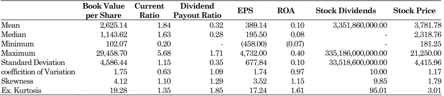
Table 2 presents the descriptive statistics for the observed variables. All variables had a common data distribution. It could thus be concluded that it was positively skewed since the number of mean is bigger than median. Some companies seem have bigger values for each variable relative to the others, indicating that the distribution of the data would exhibit positive skewness. Furthermore, it is also reveals that there is a very large dispersion of stock dividends variable. The fact that there is only one company declared and distributed dividend (Bank Pan Indonesia) in the observed that may contribute to the dispersion. This fact would potentially bias the data analysis. Consequently, this variable should be removed to secure the model.
In addition, other relatively-wide dispersions on the data occur in the book value per share and EPS variables. These dispersions could be due to the wide variability of the number of shares outstanding. For instance, the outstanding shares of Kalbe Farma ranged from 40,000 to 10,000 shares, while International Nickel Indonesia had approximately 29,000,000-190,000,000 outstanding shares.
The fluctuated performance of the companies’ share prices at that time also seems to become the major reason why the EPS experienced a relatively wide rage of discrepancy. There were three Table 2. Descriptive Statistics of Variables for the Year 2002-2006
Book Value
per Share
Current Ratio
Dividend
Payout Ratio EPS ROA Stock Dividends Stock Price
Mean 2,625.14 1.84 0.32 389.14 0.10 3,351,860,000.00 3,781.78
companies suffered from a big loss in the three periods: Holcim Indonesia, Indah Kiat Pulp & Paper, and Pabrik Kertas Tjiwi Kimia. The data also shows the dispersion of the book value per share variable. Kalbe Farma, for example, had a very small book value per share (102.70) compared to that of International Nickel Indonesia (29,458.70).
Presentation and Analysis of the Panel Data Regression Model
After completing data collecting process, the next step is to answer the research question by developing a panel regression model. Figure 1 presents the model.
To develop the model, firstly it is necessary to validate the preference of using random effect approach against naïve model by conducting the Breusch-Pagan test. The p-value, as can be seen in Figure 1, is less than 0.01, meaning that null hypothesis is not true (Lind et al., 2005), thus it should be rejected. This confirms that that there is a validation to the preference of using the random effect approach against the naïve model.
Following the Breusch-Pagan test, this study would run the Hausman test in order to validate the preference of using the random effect approach against the fixed affect approach. The null hypothesis underlying this test is that these estimates are consistent, so that the fixed effect approach and random effect approach estimators do not differ substantially. Figure 1 shows that the
p-value is less than 0.05, meaning that the null hypothesis is rejected. The conclusion is that the random effect approach is not appropriate for this study, thus the fixed effect approach may be a suitable alternative (Gujarati 2004).
Based on that fact above, this study then run a new alternative panel-data regression model by using the fixed effect approach. That alternative model is presented in the Figure 2.
Since this study come up with an alternative model, there are two panel-data regression models that have to be compared. The use of the AIC, Schwarz-BIC, and the HQC is then important. The values of the three statistics in the new model are smaller than those of the old one. It is explicitly proved that the new model have a goodness of fit and is adequate than the old one (Gujarati, 2004). Moreover, according to Cottrell and Lucchetti (2008), the smaller the value of those criteria, the better the model. From this point of view, the new panel-data regression model is more relevant to answer the research question than the old one.
Since this study estimates a panel-data regression model using fixed effects, it automatically gets an F test for the null hypothesis
that the cross-sectional units have a common intercept. Moreover, the simultaneous determination of the explanatory variables on the stock price is also tested using F test based on the null hypothesis that all regression coefficients jointly or simultaneously equal to zero. As can be seen in Figure 2, the F test results in the p-value of less than 0.01, meaning that at least one of the regressors affects the movement of the stock price.
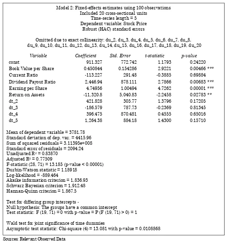
However, as can be seen in Figure 2, all firms’ dummy variables are excluded from the model because of the exact collinearity. In addition, the current ratio and all time dummy variables should be removed from the model because the variables fail to reject the null hypothesis. Consequently, the remedy for this circumstance is to run another panel-data regression model using the fixed effect approach with the exclusion of the aforementioned variables. The new model is presented by the Figure 3.
Similar to the previous models, the use of the AIC, Schwarz-BIC, and the HQC is also important. The new model have a goodness of fit and is adequate than the first and second ones (Gujarati, 2004). The values of all those criteria are the smallest. It demonstrates that the new panel-data regression model is relevant to answer the research question. The adjusted R2 indicates that the
movements of the independent variables explain 77% of the stock price variation.
After completing the F test, the model’s p -value is less than 0.01. Similar to the second model, the null hypothesis is not true, proving that at least one of the regressors could affect the movement of the stock price. Moreover, the newest model shows an improvement in the partially individual regression coefficients. After running a t test, the result shows that all independent variables have p -values of less than 0.05 rejecting the null hypotheses. It signifies that all independent variables are relevant for predicting the movement of the stock price. Nevertheless, the intercept of the model shows a p-value of more than 0.10. This describes that the presence of intercept in the model is insignificant to predict the stock price. As a result, there is no intercept included in the developed model. From the new model presented above, this study present a panel-data regression model as follow:
STOCK PRICE = 0.467752BV + 2,485.41DPR +
4.86021EPS - 13,088.3ROA (1)
Test for Plausibility and Robustness
obey as specified by the classical assumptions. However, one or more of these conditions may be violated in actual research, and this could have serious implications on the properties of the model estimators as well as the inferences drawn from them. This circumstance would make the econometrics tests unreliable. Thus, it is important to involve the test for plausibility and robustness of the developed panel-data regression model so that those ideal conditions are reasonably satisfied. Otherwise, the inferences from the model would not be valid. The tests would consist of multi-collinearity, heteroskedasticity, and autocorrelation.
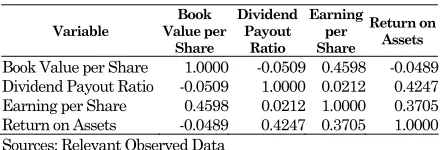
Multicollinearity could occur in the developed panel-data regression model when there is an exact linear relationship between two or more independent variables (perfect multicollinearity), or there is nearly exact linear relationship between them (near perfect multicollinearity). The multicollinearity would be detected by using the pairwise correlation among the independent variables (Danao, 2005). Strong correlations between the paired variables could result in a high degree of multicollinearity. Table 3 presents the results.
Table 3. Pairwise Correlation among the Inde-pendent Variables
Book Value per Share 1.0000 -0.0509 0.4598 -0.0489
Dividend Payout Ratio -0.0509 1.0000 0.0212 0.4247
Earning per Share 0.4598 0.0212 1.0000 0.3705
Return on Assets -0.0489 0.4247 0.3705 1.0000
Sources: Relevant Observed Data
Based on Table 3, some of the correlation coefficients indicated a relatively small relationship between the paired variables, except for the correlation between book value per share and EPS. The coefficients are still considered small because of less than 0.70 (Lind et al., 2005). However, the pairwise correlation would not detect strong linear relationships among several independent variables (Danao 2005).
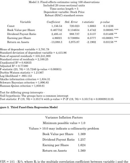
A regression of each independent variable on the rest of the others could be performed to indicate the collinearity of those regressors. A more formal way of detecting multicollinearity is to compute the variance inflation factors (VIF) of the estimated coefficients. The following figure shows the VIF of each independent variable related to the other independent variables.
The problem of multicollinearity would emerge when the value of VIF is considerably high. The higher the VIF, the more serious the multicollinearity problem (Danao 2005). The rule of thumb that is commonly used to decide whether
the problem should be concerned or not is that if the VIF’s value is less than 10, multicollinearity is not too serious. Figure 4 indicated that the VIF of all independent variables are close to one, indicating that there is multicollinearity problem.
The CLRM also includes that the variance of each disturbance term (σ2 of ui) should be constant, or homoscedastic (Gujarati 2004). Otherwise, the model would suffer from heteroskedastic problem. The problem most likely appears on cross-sectional data (Danao 2005).
The Spearman’s Rank Correlation Test (SRCT) would be employed to ensure the absence of heteroscedastic problem in the model. If the test’s computed t value exceeds its critical value, the test fails to reject the null hypothesis that the model is homoscedastic (Gujarati 2004). The Spearman's rank correlation coefficient (rho) of the model is found to be equal to -0.04996429, the computed t value and the p-value are -0.49524 and 0.6215, respectively. Consequently, by using α=5%, there is no evidence of a systematic relationship between the explanatory variable and the absolute values of the residuals, suggesting that the developed panel data regression model is free from heteroskedastic problem.
The CLRM assumes that autocorrelation should not exist in its disturbances (ui). The term autocorrelation may be defined as a correlation between members of series of observations ordered in time (as in time series data) or space (as in cross-sectional data). It could also be defined as a correlation between two time series such as u1, u2, …, u10 and u2, u3, … , u11, where the former is the latter series lagged by one time period. Since panel data have both a time-series and a cross-sectional dimension, one might expect that, in general, robust estimation of the covariance matrix would require to handle such problem (the HAC approach).
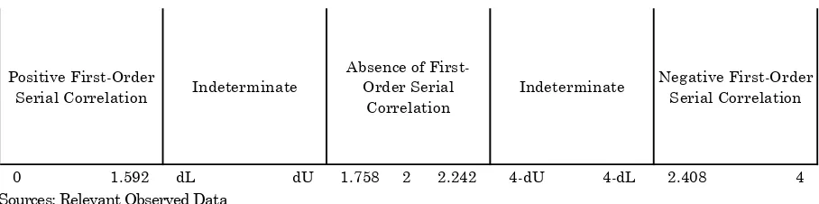
The most common test for detecting autocorrelation is the Durbin–Watson d statistic, which is simply the ratio of the sum of squared differences in successive residuals to the RSS. It worth noting that the numerator of the d statistic
is n−1 because one observation is lost in taking
successive differences (Gujarati, 2004).
As it can be seen in Figure 5, the DW is 1.214. Tabulated lower d-value (dL) for 5% significance level with four explanatory variables and 100 observations is 1.592, while the tabulated upper d -value (dU) is 1.758. Accordingly, this following figure became the basis for this study to come with the decision regarding the presence of autocorrelation problem.
autocorrelation in the model. Figure 5 shows that the computed DW is laid on the area where the null hypothesis is rejected. Therefore, the model suffers from autocorrelation problem. However, this presence of autocorrelation may not bring a serious problem to the model. Gujarati (2004) proposes to continue to use the panel-data regression model. The residual autocorrelation is not such a much property of the data, as a symptom of an inadequate model (Cottrell & Lucchetti20 08). Moreover, the estimated covariance matrix seems asymptotically valid, in term of HAC (heteroskedasticity and autocorrelation consistent).
Discussion
This study is not presenting the regression results by including time and firm’s dummy variables, for all the individual time dummies are not individually significant, and all individual firm’s dummies are omitted because of the present of perfect multocollinearity. It suggests that the year or time effect is not significant. This might suggest that the stock price would not change much over time.
Shareholder and Return-on-investment Ratios Determination on the Stock Price
The presence of shareholders’ ratios (book value per share, dividend payout ratio, and earning per share) and return-on-investment ratios (indicated by ROA) as the explanatory variables in the panel-data regression model (Formula 1) amplify the characteristics of the JSX’s investors who are interested in the return on their investments (Subiyantoro & Andreyani, 2003). The very small p-value of those independent variables, except dividend payout ratio and ROA variables, indicated that the investors prefered the LQ45’s shares to optimize the use of the own capital in generating profits. The investors also wanted a progressive growth of profits. The higher the shareholders’ ratios of the company, the more interested the investors. Moreover, it is worth noting that companies with good records of accomplishment on respect for minority shareholders’ rights and quality information disclosure were likely to find greater favor with investors (Sugiharto et al., 2007). The issues related to minority shareholders’ rights mattered during the financial crisis, and became a significant risk for the investors. Looking ahead, the investors were likely to focus on the firms’ performance regarding to the minority shareholders.
Significant statistics and positive determination of the book value per share on the stock price are consistent with those of Brief and Zarowin (1999). The difference is that Brief et. al (1999) found that book value have a greater explanatory power for stock price than the other variables. However, the consistent p-value, which is close to the 0.001, is similar to that of Brief et al (1999).
A positive coefficient of the book value per share indicates that this variable held a positive relation with the movement of the stock price at that time. The investors were willing to pay higher-price stock if the guarantee or the claim value on the companies’ net assets are presumably higher. This is due to that the book value per share describes the historical set up cost and the assets of the companies. The LQ45’s companies were believed to do their business well and efficiently, hence they could enjoy a relatively high profit so that they would eventually have a high book value.
The companies, such as Astra International, Gudang Garam, Indosat, and International Nickel Indonesia, with a relatively high book value, were able to have positive responses from investors indicated by the companies’ relatively high stock price. Unilever Indonesia, however, had very good figures on its stock price even though it did not record a high book value per share. The well brand image and the maintained good performance seemed to be the main reasons for this.
Similar to the book value per share, a positive coefficient of regression and a small p-value indicate the strong explanatory power of the dividends payout ratio to the movement of the stock price. This result is consistent with the previous research (Campbell & Shiller 1988; Nasseh & Strauss 2002). Those research have the same output, particularly when it is measured over several years.
According to Peterson and Fabozzi (2006), for the companies that pay dividends, changes in dividends are viewed favorably and associated with increases in the company’s stock price. Whereas decreases in the dividend payout ratio are viewed quite unfavorable and associated with decreases in the company’s stock price. This somewhat confirms the result of this study.
As it is mentioned above, the variable that may validly predict the stock price in this study is the EPS. It is consistent with which is reported by Conroy et. al. (2000), which states that share price reactions are significantly affected by earnings surprises, especially management forecasts of next year EPS. With positive relationship and small p -value, those research strengthen the attraction of this earning element to the JSX’s investors. The belief that the EPS has strongly influence on the stock price together with the frequent stock price reactions to earnings announcements become the reason of why earnings dominate the way of thinking in public companies as well as in the investment community. The EPS is the most widely spoken language in the financial community (Rappaport & Mauboussin, 2001).
Since the JSX’s common investors, except the government as the preferred shareholder of some formerly state-owned companies, the EPS as the figure that is left over for them is the most interested thing. It supports Ball and Shivakumar’s (2006) finding that conventional investor will focus on the firm’s EPS. Astra International, Gudang Garam, and Unilever Indonesia became the role model of how the constantly high EPS was reflected in a high and positive trend of the stock price.
Most of the companies in this study are categorized as very heavily asset companies. They do their business with the supporting of more assets compare to the others. This fact could be revealed from their ROA which was mostly less than five percent. The facts could be the reason of why the coefficient of regression of the ROA is negative. It is inconsistent with which was reported by Subiyantoro and Andreyani (2003). For the companies, the presence of many assets would reduce the ratio. However, the companies still experienced relatively high stock price presumably due to the investors’ focus which interested in the net income figure only, instead of the ratio as general.
The Absence of the Other Accounting Ratios
As seen in the data analysis section, some ratios are eliminated from the developed model because of the lousy statistics measurement, especially the p-value. This result is similar with Subiyantoro et al’s (2003). Since the object of the research is quite different with the other research, it could indicate that the JSX’s investors were not too interested in the ratios. Moreover, it should be noticed that the presence of the liquidity ratio and the stock dividends was not as attractive as the shareholders’ ratios and return-on-investment
ratio. In the relatively conventional market like Indonesia, such ratios seem to be used by the stakeholders only, but not by investors, such as banks and creditors. As it is mentioned in the data presentation, the fact that investors prefer to received cash than stock dividends made only one company that declared and distributed the dividends over the observation period.
Even though the ratios are simple and convenient, there are some shortcomings that cause the JSX’s investors would not rely on the ratios (Kieso et. al., 2001), such as: 1) the basis on the historical cost could lead to distortions in measuring performance, 2) where the estimated items are significant, income ratios lose some of their credibility, 3) the difficult problem of achieving comparability among firms in a given industry, 4) a substantial amount of important information is not included in the company’s financial statements.
CONCLUSION
The objectives of this study are to develop a particular model that shows the determination of the accounting ratios in the stock price movement. Specifically, it is aimed to find out the composition of the independent variables according to the descriptive statistics. It also requires to test which determinants (the accounting ratios) that significantly affect the most actively traded stocks in the ISX. This study also try to describe the significant contribution of the companies’ stock price consecutively classified as the LQ45 during 2002-2006 to explain the movement of the stock price in the ISX.
This study employs a secondary data of the LQ45’s companies obtained from the JSX’s official website. Some extended data gatherings are done from the exchanges counterparts to complete the value of each variable.
This study optimizes the panel-data regression model with the random approach by the supporting of econometrics package, GRETL 1.7.6. This model could be used to validly predict the movement of the stock price so that the research question regarding the significant independent variables could be answered.
2004). It indicates the preference of the investors in the ISX regarding the type of the distributed dividends, 3) Most of the dispersion of the data gathered is caused by the fluctuating performance of each company. At least there are three companies were recorded loss for some successive periods after experiencing a significant upturn in previous periods. However, these companies could still maintain their positions in the ISX’s blue chip stocks list, 4) It had already seen that the individual year effects were statistically insignificant. It indicates that the stock price had not changed much over the time period, 5) It could be said that the ISX’s investors were not concern on the accounting ratios other than the shareholders’ ratios. They implicitly placed themselves as conventional shareholders because they are only interested in the earning elements of the companies.
Based on the findings above and the new developed panel-data regression model, the accounting ratios that could determine the LQ45 stock price in the ISX during the period of 2002-2006 were book value per share, dividend payout ratio, EPS, and ROA. The ratios are classified as shareholders’ and return-on-investment ratios. Most of such variables are positive determinants on stock price, except the ROA. All of those explanatory variables showed significant influence on stock price.
The developed model shows the determination of the accounting ratios in the stock price movement . This finding could also explain the role of the LQ45 companies as the benchmark for the investors in predicting the stock price movements in the ISX generally.
Based on the conclusion above, it recommends that: 1) The BAPEPAM as the Indonesian capital market supervisor should consider to maintain and improve the performance of the ISX by encouraging more companies to list their shares in the stock exchange so that the investment preference for the investors will not be relied on the current listed companies. There should be an incentive given to pursue that objective. As noted before, most of the listed companies are family-owned ones. It indicated that the other unlisted companies could follow that pattern and did not want to sell their stocks to public. They would go public if only they want to find the other types or area of business. Moreover, the availability and adequacy of the data should be maintained and improved over times. As stated by Sugiharto et. al. (2007), most of the investors are seeking greater disclosure for listed Indonesian firms, along with
an improvement in the regulatory systems. Such improvements can reasonably be expected to increase the volition with which investors perceive LQ45 stocks, and it lies wholly within the capabilities of the relevant state bodies to make substantial positive advances in that particular area, 2) The LQ45 stock price movement could be used by the investors as the benchmark for the general stock price movement in the ISX. Most of the the LQ45’s companies can maintain their position in the blue chips classification. Moreover, the composite index’s movement was close to the LQ45 index’s. It could magnify the significant information contained in those companies’ financial statements, 3) The panel-data regression model is the simple but powerful tool to predict the movement of the stock price over some periods. However, the preference for the approach used should carefully be validated before analyzing the developed model. The presence of more variables and observations should improve the plausibility and the robustness of the model. The interrelated indices among stock exchanges in the South East Asia as described by Atmadja (2005) could be the main consideration to use the developed model in this study in predicting the stock price movement in that particular region.
REFERENCES
Atmadja, A. S. (2005). Are the five ASEAN stock price indices dynamically interacted? Jurnal Akuntansi & Keuangan (Journal of Accounting & Finance), 7 (1), 43- 60.
Ball, R., & Shivakumar, L. (2006). Earnings quality at initial public offerings: Managerial opportunism, or public-firm conservatism? Retrieved March 5, 2007, from http://usc.edu/ schools/business/FBE/seminars/papers/ipo_e rn_2006_03_22.doc
Brief, R. P., & Zarowin, P. (1999). The value relevance of dividends, book value and earnings. Retrieved February 11, 2008, from http://papers.ssrn.com/sol3/papers.cfm?abstr act_id=173629
Campbell, J. Y., & Shiller, R. J. (1988). Stock prices, earnings, and expected dividends.
The Journal of Finance, 43 (3), 661-676. Conroy, R. M., Eades, K. M., & Harris, R. S. (2000).
Cottrell, A., & Lucchetti, R. J. (2008). Gretl user’s guide: Gnu regression, econometrics, and time-series.
Danao, R. (2005). Introduction to statistics and econometrics. Manila: The University of the Philippines Press.
Dong, M. (2000). A general model of stock valuation. Retrieved February 11, 2008, from http://fisher.osu.edu/fin/students/dong/ papers/general.pdf.
Gujarati, D. (2004). Basic econometrics (4th ed.).
New York: McGraw-Hill/Irwin.
Gupta, J. P., Chevalier, A., & Sayekt, F. (2000). The causality between interest rate, exchange rate, and stock price in emerging markets: the case of the Jakarta stock exchange. Retrieved February 11, 2008, from http://papers.ssrn.com/sol3/papers.cfm?abstr act_id=251253.
Kieso, D. P., Weygandt, J. J., & Warfield, T. D. (2001). Intermediate accounting (10th ed.).
New York: John Wiley & Sons, Inc.
Kiplinger’s Personal Finance Magazine. (2005). The basics for investing in stocks. Retrieved February 11, 2008, from http://www.dfi. wa.gov/sd/pdf/ipt/stocks.pdf.
Lind, D. A., Marchal, W. G., & Wathen, S. A. (2005). Statistical techniques in business & economics(twelfth ed.). New York: McGraw-Hill/Irwin.
Nasseh, A., & Strauss, J. (2004). Stock prices and dividend discount model: Did their relation break down in the 1990s? The Quarterly Review of Economics and Finance, 44 (2), 191-207.
Peranginangin, Y. A. (2007). Leverage effect on the Jakarta stock exchange (JSX); An investigation using indices data from 1999 to 2004. Retrieved February 11, 2008, from http://ssrn.com/abstract=977337.
Peterson, P. P., & Fabozzi, F. J. (2006). Analysis of financial statements (2nd ed.). New Jersey:
John Wiley & Sons, Inc.
Rappaport, A., & Mauboussin, M. J. (2001). The trouble with earnings and price/earnings multiples. Retrieved February 11, 2008, from http://www.expectationsinvesting.com/ pdf/earnings.pdf.
Subiyantoro, E., & Andreani, F. (2003). Analisis faktor-faktor yang mempengaruhi harga saham [The analysis of the factors that influence the stock price]. Jurnal
Mana-jemen dan Kewirausahawan (Journal of
Management and Entrepreneurship), 5, 173-174.
Sources: Relevant Observed Data
Figure 1. First Panel-Data Regression Model
Model 1: Random-effects (GLS) estimates using 100 observations Included 20 cross-sectional units
Time-series length = 5 Dependent variable: Stock Price
Variable Coefficient Std. Error t-statistic p-value
const 505.515 736.366 0.6865 0.49409
Book Value per Share 0.292119 0.0742032 3.9367 0.00016 ***
Current Ratio -71.9672 261.664 -0.2750 0.78389
Dividend Payout Ratio 3,910.37 870.23 4.4935 0.00002 ***
Earning per Share 3.61727 0.500393 7.2289 <0.00001 ***
Return on Assets -132.25 4,042.45 -0.0327 0.97397
Mean of dependent variable = 3,781.78
Standard deviation of dependent variable = 4,415.96 Sum of squared residuals = 632,876,000
Standard error of residuals = 2,581.06 'Within' variance = 4,469,880
'Between' variance = 2,932,110
Theta used for quasi-demeaning = 0.44783 Akaike information criterion = 1,861.85 Schwarz Bayesian criterion = 1,877.48 Hannan-Quinn criterion = 1,868.18
Breusch-Pagan test -
Null hypothesis: Variance of the unit-specific error = 0
Asymptotic test statistic: Chi-square (1) = 7.71828 with p-value = 0.00546645
Hausman test -
Null hypothesis: GLS estimates are consistent
Sources: Relevant Observed Data
Figure 2. Second Panel-Data Regression Model
Model 2: Fixed-effects estimates using 100 observations Included 20 cross-sectional units
Time-series length = 5 Dependent variable: Stock Price
Robust (HAC) standard errors
Omitted due to exact collinearity: du_2, du_3, du_4, du_5, du_6, du_7, du_8, du_9, du_10, du_11, du_12, du_13, du_14, du_15, du_16, du_17, du_18, du_19, du_20
Variable Coefficient Std. Error t-statistic p-value
const 911.327 772.742 1.1793 0.24220
Book Value per Share 0.450844 0.154286 2.9221 0.00466 ***
Current Ratio -113.227 291.48 -0.3885 0.69884
Dividend Payout Ratio 2,446.94 878.111 2.7866 0.00683 ***
Earning per Share 4.74956 1.00494 4.7262 0.00001 ***
Return on Assets -11,320.8 5,040.83 -2.2458 0.02783 **
dt_2 421.828 305.77 1.3796 0.17205
dt_3 -186.579 787.73 -0.2369 0.81345
dt_4 396.475 870.481 0.4555 0.65016
dt_5 1,264.38 884.18 1.4300 0.15710
Mean of dependent variable = 3781.78 Standard deviation of dep. var. = 4415.96 Sum of squared residuals = 3.11395e+008 Standard error of residuals = 2094.24 Unadjusted R2 = 0.83870
Adjusted R2 = 0.77509
F-statistic (28, 71) = 13.185 (p-value < 0.00001) Durbin-Watson statistic = 1.18918
Log-likelihood = -889.464
Akaike information criterion = 1,836.93 Schwarz Bayesian criterion = 1,912.48 Hannan-Quinn criterion = 1,867.5
Test for differing group intercepts -
Null hypothesis: The groups have a common intercept
Test statistic: F (19, 71) = 0 with p-value = P (F (19, 71) > 0) = 1
Wald test for joint significance of time dummies
Figure 3. Third Panel-Data Regression Model
Figure 4. VIF of the Independent Variables
Model 3: Fixed-effects estimates using 100 observations Included 20 cross-sectional units
Time-series length = 5 Dependent variable: Stock Price
Robust (HAC) standard errors
Variable Coefficient Std. Error t-statistic p-value
Const 1,156.54 720.023 1.6063 0.11236
Book Value per Share 0.467752 0.134634 3.4742 0.00085 *** Dividend Payout Ratio 2,485.41 988.737 2.5137 0.01406 ** Earning per Share 4.86021 0.738894 6.5777 <0.00001 *** Return on Assets -13,088.3 5,975.87 -2.1902 0.03158 **
Mean of dependent variable = 3,781.78
Standard deviation of dependent variable = 4,415.96 Sum of squared residuals = 335,241,000
Standard error of residuals = 2,100.25 Unadjusted R2 = 0.82635
Adjusted R2 = 0.77380
F-statistic (23, 76) = 15.7246 (p-value < 0.00001) Durbin-Watson statistic = 1.21367
Log-likelihood = -893.153
Akaike information criterion = 1,834.31 Schwarz Bayesian criterion = 1,896.83 Hannan-Quinn criterion = 1,859.61
Test for differing group intercepts -
Null hypothesis: The groups have a common intercept
Test statistic: F (19, 76) = 3.35174 with p-value = P (F (19, 76) > 3.35174) = 0.0000913135
Variance Inflation Factors Minimum possible value = 1.0
Values > 10.0 may indicate a collinearity problem Book Value per Share 1.369
Dividend Payout Ratio 1.257 Earning per Share 1.624 Return on Assets 1.560
VIFj = 1/(1 - Rj2), where Rj is the multiple correlation coefficient between variable j and the other independent variables
Properties of matrix X'X: 1-norm = 3,015,681,500
Determinant = 50,897,612,000,000,000,000
Positive First-Order
Serial Correlation Indeterminate
Absence of First-Order Serial
Correlation
Indeterminate Negative First-Order Serial Correlation
0 1.592 dL dU 1.758 2 2.242 4-dU 4-dL 2.408 4 Sources: Relevant Observed Data