Academic Press Digital Signal Processing System Design 2nd Edition Apr 2008 ISBN 0123744903 pdf

(1)

(2)

Digital Signal Processing System

Design: LabVIEW-Based Hybrid

Programming

(3)

(4)

Digital Signal Processing System

Design: LabVIEW-Based Hybrid

Programming

by Nasser Kehtarnavaz

University of Texas at Dallas

With laboratory contributions by Namjin Kim

and Qingzhong Peng

Amsterdam • Boston • Heidelberg • London • New York • Oxford Paris • San Diego • San Francisco • Singapore • Sydney • Tokyo

(5)

Academic Press is an imprint of Elsevier

30 Corporate Drive, Suite 400, Burlington, MA 01803, USA 525 B Street, Suite 1900, San Diego, California 92101-4495, USA 84 Theobald’s Road, London WC1X 8RR, UK

Cover image: supplied by author Cover Design: Alisa Andreola Cover Direction: Alisa Andreola

No part of this publication may be reproduced or transmitted in any form or by any means, electronic or mechanical, including photocopy, recording, or any information storage and retrieval system, without permission in writing from the publisher.

Permissions may be sought directly from Elsevier’s Science & Technology Rights Department in Oxford, UK: phone: (_þ44) 1865 843830, fax: (_þ44) 1865 853333, E-mail: permissions@elsevier.com. You may also complete your request online via the Elsevier homepage (http://elsevier.com), by selecting “Support & Contact” then “Copyright and Permission” and then “Obtaining Permissions.”

Library of Congress Cataloging-in-Publication Data

Application Submitted

British Library Cataloguing-in-Publication Data

A catalogue record for this book is available from the British Library. ISBN: 978-0-12-374490-6

(6)

Preface

The previous edition of this book, titledDigital Signal Processing System-Level

Design Using LabVIEW, showed how LabVIEWTM graphical programming can be

used to build and analyze digital signal processing (DSP) systems in an interactive manner and in relatively shorter times as compared to text-based programming. The motivation for writing the previous edition was derived from the observation that many students taking DSP lab courses, in particular at the undergraduate level,

often struggle and spend a fair amount of their time debugging C and MATLABW

codes in lab sessions instead of placing more effort into analyzing and thus understanding signal processing systems.

In this second edition of the book, graphical and textual programming are combined to provide a hybrid programming approach toward achieving a more effective mechanism to build and analyze DSP systems. Textual programming and graphical programming have their own merits and demerits from a programming point of view. In general, math operations are found to be easier to code in textual mode. For example, MATLAB provides a rich set of built-in functions for performing signal processing vector and matrix-based math operations. On the other hand, graphical programming offers an easy-to-build interactive and visualization environment and a more intuitive approach toward building signal processing systems.

In an effort to bring together the preferred features of textual and graphical

(13)

In addition to the hybrid programming approach adopted in this second edition, the labs have been redesigned based on the latest release of LabVIEW (LabVIEW 8.5) at the time of this writing instead of LabVIEW 7.1, which was utilized in the first edition.

I would like to express my appreciation and gratitude to National Instruments, in particular the Academic Marketing Division, for their support of this book.

Nasser Kehtarnavaz December 2007

(14)

What’s On the CD-ROM?

The accompanying CD-ROM includes all the lab files discussed throughout the book. These files are placed in corresponding folders as follows:

○ Lab01: Getting Familiar with LabVIEW: Part I ○ Lab02: Getting Familiar with LabVIEW: Part II ○ Lab03: Sampling, Quantization, and Reconstruction ○ Lab04: FIR/IIR Filtering System Design

○ Lab05: Data Type and Scaling ○ Lab06: Adaptive Filtering Systems ○ Lab07: FFT, STFT, and DWT

○ Lab08: Getting Familiar with Code Composer Studio ○ Lab09: DSP Integration Examples

○ Lab10: Hybrid Programming of Dual Tone Multi-Frequency System ○ Lab11: Hybrid Programming of 4-QAM Modem System

○ Lab12: Hybrid Programming of Cochlear Implant Simulator System

(15)

For Lab 8 and Lab 9, the Texas Instruments Code Composer StudioTM(CCStudio) version 3.0 is used and assumed installed in the folder “C:\CCStudio\”. The subfolders correspond to the following DSP platforms:

○ DSK 6416 ○ DSK 6713

○ Simulator (configured as DSK6713 as shown in the following figure)

(16)

(17)

(18)

C H A P T E R

1

Introduction

The field of digital signal processing (DSP) has experienced a considerable growth in the past two decades, primarily due to the availability and advancements in digital signal processors (also called DSPs). Nowadays, DSP systems such as cell phones and high-speed modems have become an integral part of our lives.

In general, sensors generate analog signals in response to various physical phenom-ena that occur in an analog manner (i.e., in continuous-time and amplitude). Pro-cessing of signals can be done either in analog or digital domain. To perform the processing of an analog signal in digital domain, it is required that a digital signal is formed by sampling and quantizing (digitizing) the analog signal. Hence, in contrast to an analog signal, a digital signal is discrete in both time and amplitude. The digitization process is achieved via an analog-to-digital (A/D) converter. The field of DSP involves the manipulation of digital signals in order to modify their charac-teristics or to extract useful information from them.

(19)

1.1 Digital Signal Processing Hands-On Lab Courses

Nearly all electrical engineering curricula include DSP courses. DSP lab or design courses are also being offered at many universities concurrently or as follow-ups to DSP theory courses. These hands-on lab courses have played a major role in better understanding of DSP concepts. A number of textbooks, e.g. [1–5], have been writ-ten to provide the teaching materials for DSP lab courses. The programming

lan-guage used in these textbooks consists of either C, MATLABW, or Assembly, which

are all text-based languages. In addition to these text-based languages, it is becoming important for students to gain experience in block-based or graphical (G) program-ming or environment for the purpose of designing DSP systems in a relatively short amount of time. Graphical programming offers an interactive and a more intuitive approach toward building DSP systems. Thus, the main objective of this book is to provide a block-based or system-level programming approach in DSP lab courses. The system-level programming environment chosen is LabVIEW.

Laboratory Virtual Instrumentation Engineering Workbench (LabVIEW) is a graphical programming environment developed by National Instruments (NI) which allows performing high-level or system-level designs. It uses a graphical programming language to create so-called Virtual Instrument (VI) blocks in an intuitive flowchart-like manner. A design is achieved by integrating different blocks, components, or subsystems within a graphical framework. LabVIEW provides data acquisition, analysis, and visualization features well suited for DSP system design. It is also an open environment accommodating MATLAB and C Dynamic Link Libraries (DLLs).

This book is written primarily for those who are already familiar with signal pro-cessing concepts and are interested in designing signal propro-cessing systems without needing them to be proficient C or MATLAB programmers. After familiarizing the reader with LabVIEW, the book covers a LabVIEW-based approach to generic experiments encountered in a typical DSP lab course. It brings together in one place the information scattered in several NI LabVIEW manuals to provide the necessary tools and know-how for designing signal processing systems within a one-semester lab course. This book can also be used as a self-study LabVIEW guide toward designing and analyzing signal processing systems.

In addition, for those interested in DSP hardware implementation, two chapters in the book are dedicated to executing selected portions of a LabVIEW designed system on an actual DSP processor. The DSP processor chosen is TMS320C6000. This processor has been manufactured by Texas Instruments (TI) for computationally intensive signal processing applications. The DSP hardware utilized to interface with

(20)

LabVIEW is the widely adopted TI’s C6416 or C6713 DSP Starter Kit (DSK) board. It should be mentioned that since the DSP hardware implementation aspect of the labs (which includes C programs) is independent of the LabVIEW imple-mentation, those who are not interested in the DSP hardware implementation may skip these two chapters.

1.2 Organization

The book includes 12 chapters and 12 labs. After this introduction, the LabVIEW programming environment is presented in Chapter 2. Lab 1 and Lab 2 in Chapter 2 provide a tutorial on getting familiar with the LabVIEW programming environ-ment. Lab 1 provides a general introduction to LabVIEW, and Lab 2 covers building signal processing systems graphically. Lab 2 also shows how to incorporate M-file nodes or blocks within LabVIEW. The topic of analog-to-digital signal conversion is presented in Chapter 3 followed by Lab 3 covering signal sampling experiments. Chapter 4 involves digital filtering. Lab 4 in Chapter 4 shows how to use LabVIEW to design FIR and IIR digital filters. In Chapter 5, fixed-point versus floating-point implementation issues are discussed, followed by Lab 5 covering data type and fixed-point effect experiments. In Chapter 6, the topic of adaptive filtering is dis-cussed. Lab 6 in Chapter 6 covers two adaptive filtering systems consisting of system identification and noise cancellation. Chapter 7 presents frequency domain

processing, followed by Lab 7 covering the three widely used transforms in signal processing: fast Fourier transform (FFT), short-time Fourier transform (STFT), and discrete wavelet transform (DWT). Chapter 8 discusses the implementation of a LabVIEW-designed system on the TMS320C6000 DSP processor. First, an overview of the TMS320C6000 architecture is provided. Then, in Lab 8, a tutorial is

presented to show how to use the Code Composer Studio (CCStudio) software development tool to achieve the DSP hardware implementation. As a continuation of Chapter 8, Chapter 9 and Lab 9 discuss the issues related to the interfacing of LabVIEW and the DSP processor. Chapters 10 through 12 and Labs 10 through 12, respectively, discuss the following three DSP systems or project examples that are designed in a hybrid mode or a combination of graphical and textual modes: (i) dual tone multi-frequency (DTMF) signaling, (ii) software-defined radio, and (iii) cochlear implant simulator.

1.3 Software Installation

LabVIEW 8.5, which is the latest version at the time of this writing, can be installed

by runningsetup.exe on the LabVIEW Core DVD. Some lab portions use the

(21)

Integration for TI DSP.” The toolkit “Digital Filter Design” appears under the Lab-VIEW Core DVD and can be included while installing LabLab-VIEW 8.5. The toolkits “Advanced Signal Processing” and “DSP Test Integration for TI DSP” appear on the Signal Processing and Communications DVD and can be installed by running setup.exeon this DVD. To generate C DLLs, it is required to have Microsoft Visual

StudioW or a similar C development environment installed. To use the MATLAB

script node feature of LabVIEW, it is required to have MATLAB Version 6.0 or later installed.

If one desires to run parts of a LabVIEW-designed system on a DSP processor, then it is required to install the Code Composer Studio (CCStudio) software tool by

runningsetup.exe on the CCStudio CD. In the DSK related labs, CCStudio v3.0 is

used.

The accompanying CD includes all the files necessary for running the labs covered throughout the book.

1.4 Updates

Considering that any programming environment goes through enhancements and updates, it is expected that there will be updates of LabVIEW and its toolkits. To accommodate for such updates and to make sure that the labs provided in the book can still be used in DSP lab courses, any new version of the labs will be posted at the website http://www.utdallas.edu/~kehtar/LabVIEW for easy access. It is recom-mended that this website is periodically checked to download any necessary updates.

1.5 Bibliography

[1] N. Kehtarnavaz,Real-Time Digital Signal Processing Based on the TMS320C6000, Elsevier, 2005.

[2] S. Kuo and W-S. Gan,Digital Signal Processors: Architectures, Implementations, and Applications, Prentice-Hall, 2005.

[3] R. Chassaing, DSP Applications Using C and the TMS320C6x DSK, Wiley

Inter-Science, 2002.

[4] T. Welch, C. Wright and M. Morrow, Real-Time Digital Signal Processing

from MATLAB to C with the TMS320C6x DSK, CRC Press, 2006.

[5] L. Tan,Digital Signal Processing: Fundamentals and Applications, Elsevier, 2007.

(22)

C H A P T E R

2

LabVIEW Graphical Programming

Environment

LabVIEW constitutes a graphical programming environment that allows one to design and analyze a DSP system in a shorter time as compared to text-based programming environments. LabVIEW graphical programs are called Virtual Instruments (VIs). VIs run based on the concept of data flow programming. This means that execution of a block or a graphical component is dependent on the flow of data, or more specifically a block executes when data are made available at all of its inputs. Output data of the block are then sent to all other connected blocks. Data flow programming allows multiple operations to be performed in parallel, since its execution is determined by the flow of data and not by sequential lines of code.

2.1 Virtual Instruments (VIs)

A VI consists of two major components, which include a Front Panel (FP) and a Block Diagram (BD). An FP provides the user-interface of a program, whereas a BD incorporates its graphical code. When a VI is located within the block diagram of another VI, it is called a subVI. LabVIEW VIs are modular, meaning that any VI or subVI can be run by itself.

2.1.1 Front Panel and Block Diagram

(23)

A BD contains terminal icons, nodes, wires, and structures. Terminal icons are interfaces through which data are exchanged between an FP and a BD. They correspond to controls or indicators that appear on an FP. Whenever a control or indicator is placed on an FP, a terminal icon gets added to the corresponding BD. A node represents an object which has input and/or output connectors and performs a certain function. SubVIs and functions are examples of nodes. Wires establish the flow of data in a BD. Structures are used to control the flow of a program such as repetitions or conditional executions. Figure 2-1 shows what an FP and a BD window look like.

2.1.2 Icon and Connector Pane

A VI icon is a graphical representation of a VI. It appears in the top right corner of a BD or an FP window. When a VI is inserted in a BD as a subVI, its icon gets displayed.

A connector pane defines inputs (controls) and outputs (indicators) of a VI. The number of inputs and outputs can be changed by using different connector pane patterns. In Figure 2-1, a VI icon is shown at the top right corner of the BD and its corresponding connector pane having two inputs and one output is shown at the top right corner of the FP.

Figure 2-1: LabVIEW windows: Front Panel and Block Diagram.

(24)

2.2 Graphical Environment

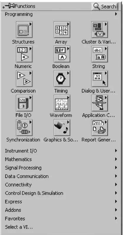
2.2.1 Functions Palette

The Functions palette, shown in Figure 2-2, provides various function VIs or blocks for building a system. This palette can be displayed by right-clicking on an open area of a BD. Note that this palette can be displayed only in a BD.

Figure 2-2: Functions palette.

(25)

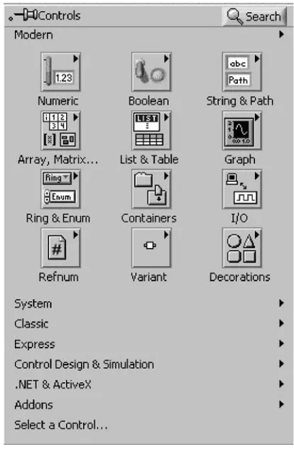
2.2.2 Controls Palette The Controls palette, shown in Figure 2-3, provides controls and indicators of an FP. This palette can be displayed by right-clicking on an open area of an FP. Note that this palette can be displayed only in an FP.

2.2.3 Tools Palette

The Tools palette provides various operation modes of the mouse cursor for building or debugging a VI. The Tools palette and the frequently used tools are shown in Figure 2-4.

Each tool is utilized for a specific task. For example, the Wiring tool is used to wire objects in a BD. If the automatic tool selection mode is enabled by clicking theAutomatic Tool Selection button, LabVIEW selects the best matching tool based on a

current cursor position. Figure 2-3: Controls palette.

Figure 2-4: Tools palette.

(26)

2.3 Building a Front Panel

In general, a VI is put together by going back and forth between an FP and a BD, placing inputs/outputs on the FP and building blocks on the BD.

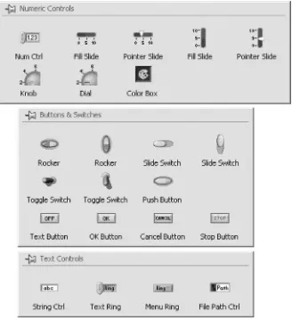
2.3.1 Controls

Controls make up the inputs to a VI. Controls grouped in the Numeric Controls palette (Controls » Express » Num Ctrls) are used for numerical inputs, grouped in the Buttons & Switches palette (Controls » Express » Buttons) for Boolean inputs, and grouped in the Text Controls palette (Controls » Express » Text Ctrls) for text and enumeration inputs.

These control options are displayed in Figure 2-5.

Figure 2-5: Control palettes.

(27)

2.3.2 Indicators

Indicators make up the outputs of a VI. Indicators grouped in the Numeric Indicators palette (Controls » Express » Num Inds) are used for numerical outputs, grouped in the LEDs palette (Controls » Express » LEDs) for Boolean outputs, grouped in the Text Indicators palette (Controls » Express » Text Inds) for text outputs, and grouped in the Graph Indicators palette (Controls » Express » Graph Indicators) for graphical outputs. These indicator options are displayed in Figure 2-6.

2.3.3 Align, Distribute, and Resize Objects

The menu items on the toolbar of an FP, as shown in Figure 2-7, provide options to align and orderly distribute objects on the FP. Normally, after controls and

indicators are placed on an FP, one uses these options to tidy up their appearance.

Figure 2-6: Indicator palettes.

(28)

2.4 Building a Block Diagram

2.4.1 Express VI and Function

Express VIs denote higher-level VIs that have been configured to incorporate

lower-level VIs or functions. These VIs are displayed as expandable nodes with a blue background. Placing an Express VI in a BD brings up a configuration window

allowing adjustment of its parameters. As a result, Express VIs demand less wiring. A configuration window can be brought up by double-clicking on its Express VI.

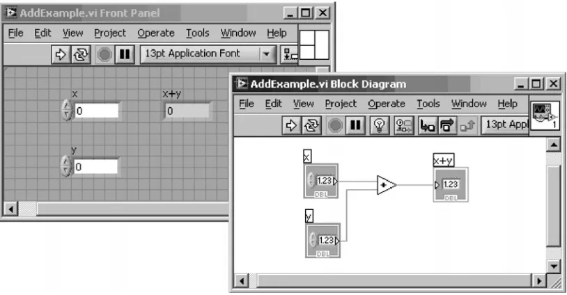
Basic operations such as addition or subtraction are represented by functions. Figure 2-8 shows three examples corresponding to three types of a BD object (VI, Express VI, and function).

A subVI or an Express VI can be displayed as icons or expandable nodes. If a subVI is displayed as an expandable node, the background appears yellow. Icons are used to save space in a BD, while expandable nodes are used to provide easier wiring or better readability. Expandable nodes can be resized to show their connection nodes more clearly. Three appearances of a VI/Express VI are shown in Figure 2-9.

Figure 2-7: Menu for align, distribute, resize, and reorder objects.

Figure 2-8: Block Diagram objects (a) VI, (b) Express VI, and (c) function.

(29)

2.4.2 Terminal Icons

FP objects get displayed as terminal icons in a BD. A terminal icon exhibits an input or output as well as its data type. Figure 2-10 shows two terminal icon examples consisting of a double precision numerical control and indicator. As shown in this figure, terminal icons can be displayed as data type terminal icons to conserve space in a BD.

2.4.3 Wires

Wires transfer data from one node to another in a BD. Based on the data type of a data source, the color and thickness of its connecting wires change.

Figure 2-9: Icon versus expandable node.

Figure 2-10: Terminal icon examples displayed in a BD.

(30)

Wires for the basic data types used in LabVIEW are shown in Figure 2-11. Other than the data types shown in this figure, there are some other specific data types. For example, the dynamic data type is always used for Express VIs, and the waveform data type, which corresponds to the output from a waveform generation VI, is a special cluster of components incorporating trigger time, time interval, and data value.

2.4.4 Structures

A structure is represented by a graphical enclosure. The graphical code enclosed by a structure gets repeated or executed conditionally. A loop structure is equivalent to aFor Loop or a While Loopstatement encountered in text-based

programming languages, whereas a Case structure is equivalent to anif-else

statement.

2.4.4.1 For Loop

AFor Loopstructure is used to perform repetitions. As illustrated in Figure 2-12, the displayed border indicates a For Loop structure, where the count terminal

represents the number of times the loop is to be

repeated. It is set by wiring a value from outside the loop

to it. The iteration terminal denotes the number of

completed iterations, which always starts at zero.

Wire Type Scalar 1D Array 2D Array Color

Orange (Floating point)

Figure 2-11: Basic types of wires [2].

Figure 2-12: For Loop.

(31)

2.4.4.2 While Loop

AWhile Loop structure allows repetitions depending on a condition; see Figure 2-13. The conditional

terminal initiates a stop if the condition is true.

Similar to a For Loop, the iteration terminal

provides the number of completed iterations, always starting at zero.

2.4.4.3 Case Structure

A Case structure, shown in Figure 2-14, allows running different sets of operations depending on the value it receives through its selector terminal, which is indicated by . In addition to Boolean type, the input to a selector terminal can be of integer, string, or enumerated type. This input determines which case to execute. The case

selector shows the status being executed. Cases

can be added or deleted as needed.

2.5 MathScript

MathScript is a new feature of the latest version of LabVIEW (LabVIEW 8.0_þ)

which allows one to perform textual programming in conjunction with graphical programming [6]. It includes various built-in functions and uses matrices and arrays as fundamental data types with built-in operators for data manipulation. User-defined functions can also be added to it. MathScript is compatible with the M-file script syntax that is encountered in MATLAB codes. MathScript possesses an interactive and a programming interface named MathScript Interactive Window and MathScript Node, respectively.

A MathScript Interactive Window is shown in Figure 2-15. Three interfaces— command window, output window, and MathScript window—are shown in this figure. The command window interface is used to enter commands and for script debugging or to view help statements for built-in functions. The output window interface is used for viewing output values. The MathScript window interface is used to display variables, edit scripts, and display command history. Script editing allows the execution of a group of commands.

A MathScript Node represents the textual code via a blue rectangle, as shown in Figure 2-16. Its inputs and outputs are defined on the border of this rectangle

Figure 2-14: Case structure. Figure 2-13: While Loop.

(32)

Figure 2-16: MathScript Node Interface. Figure 2-15: MathScript Interactive Window.

(33)

for transferring data between the graphical environment and a textual

MathScript code. For example, as indicated in Figure 2-16, the input variables

on the left side, namely lowcutoff, uppcutoff, and order, transfer

values to the M-file script and the output variables on the right side, namely

Fand sH, transfer values to the graphical environment. This process makes it

easy to utilize M-file script variables within the graphical programming environment.

2.6 Grouping Data: Array & Cluster

An array represents a group of elements having the same data type. An array consists

of data elements having a dimension up to 231–1. For example, if a random number

is generated in a loop, it makes sense to build the output as an array, since the length of the data element is fixed at 1 and the data type is not changed during iterations.

A cluster consists of a collection of different data type elements, similar to the structure data type in text-based programming languages. Clusters allow one to reduce the number of wires on a BD by bundling different data type elements together and passing them to only one terminal. An individual element can be

added to or extracted from a cluster by using the cluster functions such as Bundle

by Name andUnbundle by Name.

2.7 Debugging and Profiling VIs

2.7.1 Probe Tool

The Probe tool is used for debugging VIs as they run. The value on a wire can be checked while a VI is running. Note that the Probe tool can be accessed only in a BD window.

The Probe tool can be used together with breakpoints and execution highlighting to identify the source of an incorrect or an unexpected outcome. A breakpoint is used to pause the execution of a VI at a specific location, while execution highlighting helps one to visualize the flow of data during program execution.

2.7.2 Profile Tool

The Profile tool can be used to gather timing and memory usage information, i.e., how long a VI takes to run and how much memory it consumes. It is necessary to make sure a VI is stopped before setting up a Profile window.

(34)

An effective way to become familiar with LabVIEW programming is by going through hands-on examples. Thus, in the two labs that follow in this chapter, most of the key programming features of LabVIEW are learned via building some simple VIs. More detailed information on LabVIEW programming can be found in [1-6].

(35)

2.8 Bibliography

[1] National Instruments,LabVIEW Getting Started with LabVIEW, Part Number

323427A-01, 2003.

[2] National Instruments, LabVIEW User Manual, Part Number 320999E-01,

2003.

[3] National Instruments, LabVIEW Performance and Memory Management,

Part Number 342078A-01, 2003.

[4] National Instruments, Introduction to LabVIEW Six-Hour Course, Part

Number 323669B-01, 2003.

[5] Robert H. Bishop, Learning with LabVIEW 7 Express, Prentice-Hall, 2003.

[6] National Instruments, Inside LabVIEW MathScript, http://zone.ni.com/

devzone/conceptd.nsf/webmain

(36)

Lab 1: Getting Familiar

with LabVIEW: Part I

The objective of this first lab is to provide an initial hands-on experience in building a VI. For detailed explanations of the LabVIEW features mentioned here, the reader is referred to [1]. LabVIEW 8.5 can get launched by double-clicking on the LabVIEW 8.5 icon. The dialog box shown in Figure L1-1 should appear.

(37)

L1.1 Building a Simple VI

To become familiar with the LabVIEW programming environment, it is found to be more effective if one starts by going through a simple example. The example presented here consists of calculating the sum and average of two input values. This example is described in a step-by-step fashion in the following sections.

L1.1.1 VI Creation

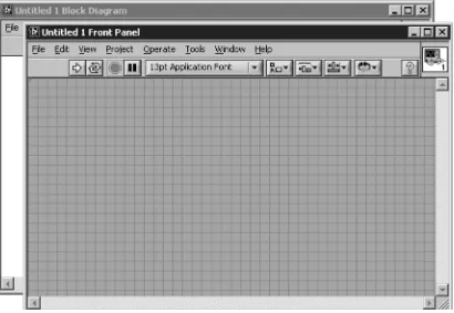
To create a new VI, click on theBlank VI under New; see Figure L1-1. This step can

also be done by choosingFile » New VI from the menu. As a result, a blank FP and a

blank BD window appear, as shown in Figure L1-2. It should be remembered that an FP and a BD coexist when building a VI.

Clearly, the number of inputs and outputs to a VI is dependent on its function. In this example, two inputs and two outputs are needed, one output generating the sum and the other the average of two input values. The inputs are created by locating twoNumeric

Figure L1-2: Blank VI.

(38)

Controlson the FP. This is done by right-clicking on an open area of the FP to bring up the Controls palette, followed by choosingControls » Modern » Numeric » Numeric Control. Each numeric control automatically places a corresponding terminal icon on the BD. Double-clicking on a numeric control highlights its counterpart on the BD, and vice versa.

Next, let us label the two inputs asxandy. This is achieved by using the Labeling tool from theToolspalette, which can be displayed by choosingView » Tools Palette

from the menu bar. Choose the Labeling tool and click on the default labels,Numeric andNumeric 2, in order to edit them. Alternatively, if the automatic tool selection mode is enabled by clickingAutomatic Tool Selectionin theToolspalette, the labels can be edited by simply double-clicking on the default labels. Editing a label on the FP

changes its corresponding terminal icon label on the BD, and vice versa.

Similarly, the outputs are created by locating twoNumeric Indicators

(Controls » Modern » Numeric » Numeric Indicator) on the FP. Each numeric indicator automatically places a corresponding terminal icon on the BD. Edit the labels

of the indicators to readSum and Average.

For a better visual appearance, objects on an FP window can be aligned, distributed, and resized using the appropriate buttons appearing on the FP toolbar. To do this, select the objects to be aligned or distributed and apply the appropriate option from the toolbar menu. Figure L1-3 shows the configuration of the FP just created.

Figure L1-3: FP configuration.

(39)

Now, let us build a graphical code on the BD to perform the summation and averaging operations. Note that<Ctrl-E>toggles between an FP and a BD window. If one finds the objects on a BD are too close to insert other functions or VIs in between, a horizontal or vertical space can be inserted by holding down the<Ctrl>

key to create space horizontally and/or vertically. As an example, Figure L1-4(b) illustrates a horizontal space inserted between the objects shown in Figure L1-4(a).

Next, place an Add function (Functions » Express » Arithmetic & Comparison » Express Numeric » Add) and aDivide function (Functions » Express » Arithmetic & Comparison » Express Numeric » Divide) on the BD. The divisor, in our case 2, needs to be entered in a Numeric Constant(Functions » Express » Arithmetic & Comparison » Express Numeric » Numeric Constant) and connected to theyterminal of theDivide function using the Wiring tool.

To have a proper data flow, functions, structures, and terminal icons on a BD need to be wired. The Wiring tool is used for this purpose. To wire these objects, point the Wiring tool at a terminal of a function or a subVI to be wired, click on the terminal, drag the mouse to a destination terminal, and click once again. Figure L1-5 illustrates the wires placed between the terminals of the numeric controls and the input terminals of the add function. Notice that the label of a terminal is displayed whenever the cursor is moved over it if the automatic tool selection mode is enabled. Also, note that the

Run button on the toolbar remains broken until the wiring process is completed.

For better readability of a BD, wires which are hidden behind objects or crossed over

other wires can be cleaned up by right-clicking on them and choosingClean Up Wire

from the shortcut menu. Any broken wires can be cleared by pressing <Ctrl-B>or

Edit » Remove Broken Wires.

The label of a BD object, such as a function, can be shown (or hidden) by

right-clicking on the object and checking (or unchecking) Visible Items » Label from the

shortcut menu. Also, a terminal icon corresponding to a numeric control or indi-cator can be shown as a data type terminal icon. This is done by right-clicking on

the terminal icon and uncheckingView As Iconfrom the shortcut menu. Figure L1-6

shows an example where the numeric controls and indicators are shown as data type terminal icons. The notation DBL represents double precision data type.

It is worth pointing out that there exists a shortcut to build the preceding VI. Instead of choosing the numeric controls, indicators, or constants from the Controls or Functions palette, one can use the shortcut menu Create, activated by right-clicking on a terminal of a BD object such as a function or a subVI. As an example of this

approach, create a blank VI and locate anAdd function. Right-click on its x

ter-minal and chooseCreate » Control from the shortcut menu to create and wire a

(40)

Figure L1-4: Inserting horizontal/vertical space: (a) creating

space while holding down the<Ctrl>key, and (b) inserted

horizontal space.

(41)

Figure L1-5: Wiring BD objects.

Figure L1-6: Completed BD.

(42)

numeric control or input. This locates a numeric control on the FP as well as a

corresponding terminal icon on the BD. The label is automatically set tox. Create

a second numeric control by right-clicking on the yterminal of the Add function.

Next, right-click on the output terminal of theAdd function and choose Create »

Indicatorfrom the shortcut menu. A data type terminal icon, labeled as x_þy, is created on the BD as well as a corresponding numeric indicator on the FP.

Next, right-click on theyterminal of the Dividefunction to choose Create »

Constant from the shortcut menu. This creates a Numeric Constant as the divisor and wires itsy terminal. Type the value 2 in the numeric constant. Right-click on

the output terminal of theDivide function, labeled as x/y, and choose Create »

Indicatorfrom the shortcut menu. In case a wrong option is chosen, the terminal does not get wired. A wrong terminal option can be easily changed by right-clicking on the terminal and choosingChange to Control orChange to Constant from the shortcut menu.

To save the created VI for later use, chooseFile » Save from the menu or press

<Ctrl-S>to bring up a dialog box to enter a name. TypeSum and Averageas the

VI name and clickSave.

To test the functionality of the VI, enter some sample values in the numeric controls on the FP and run the VI by choosingOperate » Run, by pressing<Ctrl-R>, or by clicking the Run button on the toolbar.

From the displayed output values in the numeric

indicators, the functionality of the VI can be verified.

Figure L1-7 illustrates the outcome after running the VI with two inputs 10 and 30.

L1.1.2 SubVI Creation If a VI is to be used as part of a higher level VI, its connector pane needs to be configured. A connector pane assigns inputs and outputs of a subVI to its terminals through which data are exchanged.

A connector pane can be Figure L1-7: VI verification.

(43)

displayed by right-clicking on the top right corner icon of an

FP and selectingShow

Connector from the shortcut menu.

The default pattern of a connector pane is determined based on the number of con-trols and indicators. In general, the terminals on the left side of a connector pane pattern are used for inputs, and the ones on the right side for outputs. Terminals can be added to or removed from a connector pane by right-clicking and choosingAdd Terminalor

Remove Terminalfrom the shortcut menu. If a change is to be made to the number of inputs/outputs or to the distri-bution of terminals,

a connector pane pattern can be replaced with a new one by right-clicking and choosing

Patternsfrom the shortcut menu. Once a pattern is selected, each terminal needs to be reassigned to a control or an indicator by using the Wiring tool, or by enabling the automatic tool selection mode.

Figure L1-8(a) illustrates assigning a terminal of the Sum and Average VI to a numeric control. The com-pleted connector pane is shown in Figure L1-8(b).

Figure L1-8 Connector pane: (a) assigning a terminal to a control, and (b) terminal assignment completed.

(44)

Notice that the output terminals have thicker borders. The color of a terminal reflects its data type.

Considering that a subVI icon is displayed on the BD of a higher level VI, it is important to edit the subVI icon for it to be explicitly identified. Double-clicking on the top right corner icon of a BD brings up the Icon Editor. The tools provided in the Icon Editor are very similar to those encountered in other graphical editors,

such as Microsoft Paint. An editing of the icon for the Sum and Average VI is

illustrated in Figure L1-9.

A subVI can also be created from a section of a VI. To do so, select the nodes on the BD to be included in the subVI, as shown in Figure L1-10(a). Then, chooseEdit » Create SubVI. This inserts a new subVI icon. Figure L1-10(b) illustrates the BD with an inserted subVI. This subVI can be opened and edited by double-clicking on its

icon on the BD. Save this subVI as Sum andAverage.vi. This subVI performs the

same function as the originalSum and Average VI.

In Figure L1-11, the completed FP and BD of theSum and AverageVI are shown.

Figure L1-9: Editing subVI icon.

(45)

Figure L1-10 Creating a subVI: (a) selecting nodes to make a subVI, and (b) inserted subVI icon.

(46)

L1.2 Using Structures and SubVIs

Let us now consider another example to demonstrate the use of structures and subVIs. In this example, a VI is used to show the sum and average of two input values in a continuous fashion. The two inputs can be altered by the user. If the average of the two inputs becomes greater than a preset threshold value, an LED warning light is lit.

As the first step to build such a VI, build an FP as shown in Figure L1-12(a). For the inputs, consider two Knobs (Controls » Modern » Numeric » Knob). Adjust the size of the knobs by using the Positioning tool. Properties of knobs such as precision and data type can be modified by right-clicking and choosingPropertiesfrom the shortcut

menu. A Knob Properties dialog box is brought up, and an Appearance tab is

shown by default. Edit the label of one of the knobs to readInput 1. Select the

Data Rangetab, and click Representation to change the data type from double precision to byte by selectingByte among the displayed data types. This can also be

achieved by right-clicking on the knob and choosingRepresentation » Byte from

the shortcut menu. In theData Range tab, a default value needs to be specified.

Figure L1-11: Sum and Average VI.

(47)

In this example, the default value is considered to be 0. The default value can be set by right-clicking on the control and choosing Data Operations » Make Current Value Defaultfrom the shortcut menu. Also, this control can be set to a default value by right-clicking and choosingData Operations » Reinitialize to Default Value from the shortcut menu.

Label the second knob as Input 2 and repeat all the adjustments as done for the

first knob except for the data representation part. The data type of the second knob is specified to be double precision in order to demonstrate the difference in the outcome. As the final step of configuring the FP, align and distribute the objects using the appropriate buttons on the FP toolbar.

To set the outputs, locate and place aNumeric Indicator, aRound LED

(Controls » Modern » Boolean » Round LED), and aGauge(Controls » Modern » Numeric » Gauge). Edit the labels of the indicators as shown in Figure L1-12(a).

Now let us build the BD as shown in Figure L-12(b). There are five control and indicator icons already appearing on the BD. Right-click on an open area of the BD to bring up theFunctionspalette and then choose Select a VI. . ._{. This brings up a file}

Figure L1-12: Example of structure and subVI: (a) FP and (b) BD.

(48)

dialog box. Navigate to the Sum and Average VI in order to place it on the BD. This subVI is displayed as an icon on the BD. Wire the numeric controls, Input 1 andInput 2, to thexand yterminals, respectively. Also, wire theSum

terminal of the subVI to the numeric indicator labeled Sum and theAverage

terminal to the gauge indicator labeledAverage.

AGreater or Equal?function is located fromFunctions » Programming »

Comparison » Greater or Equal?in order to compare the average output of the subVI with

a threshold value. Create a wire branch on the wire between theAverageterminal

of the subVI and its indicator via the Wiring tool. Then, extend this wire to the

xterminal of theGreater or Equal?function. Right-click on theyterminal of the

Greater or Equal?function and chooseCreate » Constantin order to place a Numeric Constant. Enter 9 in the numeric constant. Then, wire theRound LED, labeled asWarning, to the

x>_¼y?terminal of this function to provide a Boolean value.

In order to run the VI

con-tinuously, one uses aWhile

Loopstructure. Choose

Functions » Programming » Structures » While Loopto

create aWhile Loop.

Change the size by dragging the mouse to enclose the

objects in theWhile Loop

as illustrated in Figure L1-13.

Once this structure is cre-ated, its boundary together with the loop iteration

terminal , and conditional

terminal get shown on

the BD. If the While Loop

is created by usingFunctions » Programming » Structures » While Loop, then the

Stop Button is not

included as part of the Figure L1-13: While Loop enclosure.

(49)

structure. This button can be created by right-clicking on the conditional terminal

and choosingCreate » Control from the shortcut menu. A Boolean condition can be

wired to a conditional terminal, instead of a stop button, in order to stop the loop programmatically.

As the final step, tidy up the wires, nodes, and terminals on the BD using the Align object and Distribute objectoptions on the BD toolbar. Then, save the VI in a file

named Structure and SubVI.vi.

Now run the VI to verify its functionality. After clicking the Run button on the toolbar, adjust the knobs to alter the inputs. Verify whether the average and sum are displayed correctly in the gauge and numeric indicators. Note that only integer values can be

entered via theInput 1knob, whereas real values can be entered via theInput

2knob. This is due to the data types associated with these knobs. TheInput 1 knob is set to byte type, i.e.,

I8 or 8-bit signed integer. As a result, only integer values within the range

128 and 127 can be entered. Considering that the minimum and

maximum value of this knob are set to 0 and 10, respectively, only

integer values from 0 to 10 can thus be entered for this input.

When the average value of the two inputs becomes greater than the preset threshold value of 9, the warning LED will light up, as shown in Figure L-14.

Click thestop buttonon

the FP to stop the VI. Otherwise, the VI keeps running until the conditional

terminal of theWhile Loop

becomes true. Figure L1-14: FP as VI runs.

(50)

L1.3 Create an Array with Indexing

Auto-indexing enables one to read/write each element from/to a data array in a loop structure. In this section, this feature is covered.

Let us first locate aFor Loop (Functions » Programming » Structures » For Loop). Right-click on its count terminal and choose Create » Constant from the shortcut menu to set the number of iterations. Enter 10 so that the code inside it gets repeated 10 times. Note that the current loop iteration count, which is read from the iteration terminal, starts at index 0 and ends at index 9.

Place aRandom Number (0–1) function (Functions » Programming » Numeric »

Random Number (0–1)) inside theFor Loop and wire the output terminal of this

function, number (0 to 1), to the border of the For Loop to create an output

tunnel. The tunnel appears as a box with the array symbol [ ] inside it. For a For Loop, auto-indexing is enabled by default, whereas for aWhile Loop, it is disabled by default. Create an indicator on the tunnel by right-clicking and choosingCreate » Indicatorfrom the shortcut menu. This creates an array indicator icon outside the loop structure on the BD. Its wire appears thicker due to its array data type. Also, another indicator representing the array index gets displayed on the FP. This indi-cator is of array data type and can be resized as desired. In this example, the size of the array is specified as 10 to display all the values, considering that the number of iterations of theFor Loop is set to be 10.

Create a second output tunnel by wiring the output of theRandom Number (0–1)

function to the border of the loop structure; then right-click on the tunnel and

chooseDisable indexingfrom the shortcut menu to disable auto-indexing. When one

does this, the tunnel becomes a filled box representing a scalar value. Create an indicator on the tunnel by right-clicking and choosingCreate » Indicator from the shortcut menu. This sets up an indicator of scalar data type outside the loop structure on the BD.

Next, create a third indicator on theNumber (0 to 1) terminal of the Random

Number (0–1) function located in theFor Loop to observe the values coming out. To do this, right-click on the output terminal or on the wire connected to this

terminal and chooseCreate » Indicator from the shortcut menu.

Place aTime DelayExpress VI (Functions » Programming » Timing » Time Delay) to delay the execution in order to have enough time to observe a current value.

A configuration window is brought up for specifying the delay time in seconds. Enter the value 0.1 to wait 0.1 seconds at each iteration. Note that theTime DelayExpress VI is shown as an icon in Figure L1-15 in order to have a more compact display.

(51)

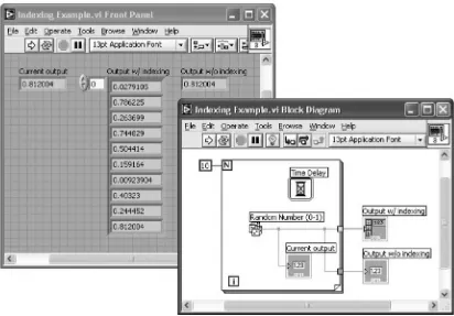
Save the VI as Indexing Example.vi and run it to observe its functionality. From the output displayed on the FP, a new random number should get displayed every 0.1 second on the indicator residing inside the loop structure. However, no data will be available from the indicators outside the loop structure until the loop iterations end. An array of 10 elements should be generated from the indexing-enabled tunnel, while only one output, the last element of the array, should be passed from the indexing-disabled tunnel.

L1.4 Debugging VIs: Probe Tool

The Probe tool is used to observe data that are being passed while a VI is running. A probe can be placed on a wire by using the Probe tool or by right-clicking on a

wire and choosingProbe from the shortcut menu. Probes can also be placed while

a VI is running.

Figure L1-15: Creating array with indexing.

(52)

Placing probes on wires creates probe windows through which intermediate values can be observed. A probe window can be customized. For example, showing data of array data type via a graph makes debugging easier. To do this, right-click on the

wire where an array is being passed and choose Custom Probe » Controls » Modern »

Graph » Waveform Graph from the shortcut menu.

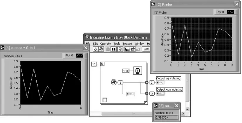
As an example of using custom probes, aWaveform Chart is used here to track

the scalar values at probe location 1, a waveform graph to monitor the array at probe location 2, and a regular probe window at probe location 3 to see the values of theIndexing Example VI. These probes and their locations are illustrated in Figure L1-16.

Figure L1-16: Probe tool.

(53)

L1.5 Bibliography

[1] National Instruments, LabVIEW User Manual, Part Number 320999E-01,

2003.

L1.6 Lab Experiments

Perform the following experiments with and without using the MathScript feature of LabVIEW 8.

1. Build a subVI to compute the product, sum, and difference of two given square

matrices A andB.

2. Build a subVI to compute and display the roots of a quadratic equation

ax2 _þ _bx _þ _c _{for given coefficients} _{a, b,} _and _c_.

3. Build a subVI to generate the first 20 numbers of the Fibonacci sequence and

store them using an indexing array.

4. Build a subVI to compute the sum of the firstn natural numbers for a specified value ofn.

(54)

Lab 2: Getting Familiar

with LabVIEW: Part II

Now that an initial familiarity with the LabVIEW programming environment has been acquired in Lab 1, this second lab shows how a DSP system can be built in LabVIEW. In addition, the hybrid programming approach is introduced.

L2.1 Express VIs Versus Regular VIs

A simple DSP system consisting of signal generation and amplification is covered here. The shape of the input signal (sine, square, triangle, or saw tooth) as well as its frequency and gain are altered by using appropriate FP controls. The system is built with Express VIs first; then the same system is built with regular VIs. This is done in order to illustrate the use of Express VIs versus regular VIs for building a system.

L2.1.1 Building a System VI with Express VIs

The use of Express VIs allows less wiring on a BD. Also, it provides an interactive user interface by which parameter values can be adjusted on the fly. The BD of the signal generation system using Express VIs is shown in Figure L2-1.

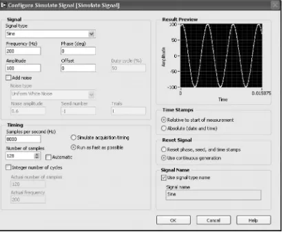
To build this BD, locate theSimulate Signal Express VI (Functions » Express

» Input » Simulate Signal) to generate a signal source. This brings up a configura-tion window, as shown in Figure L2-2. Different types of signals including sine, square, triangle, sawtooth, or DC can be generated with this VI. Enter and adjust the parameters as indicated in Figure L2-2 to simulate a sinewave having a frequency of 200 Hz and an amplitude swinging between –100 and 100. Set the sampling frequency to 8000 Hz. A total of 128 samples spanning a time duration of 15.875 milliseconds (ms) is generated. Note that when the parameters

are changed, the modified signal gets displayed instantly in the Result Preview

graph window.

Next, place a Scaling and MappingExpress VI (Functions » Express » Arithmetic

(55)

When its configuration dialog box is brought up, as shown in Figure L2-3, choose

Linear (Y=mx+b) and enter 5 inSlope (m) to scale the signal 5 times.

Wire the Sineterminal of the Simulate Signal Express VI to the Signals

terminal of the Scaling and MappingExpress VI. Note that a wire having a

dynamic data type gets created.

To display the output signal, place a waveform graph (Controls » Modern » Graph » Waveform Graph) on the FP. The waveform graph can also be created by

right-clicking on theScaled Signals terminal and choosingCreate » Graph Indicator

from the shortcut menu.

Now, in order to observe the original and the scaled signal together in the same

graph, wire the Sineterminal of the Simulate Signal Express VI to the

waveform graph. This inserts a Merge Signalsfunction on the wire

automati-cally. An automatic insertion of theMerge Signalsfunction occurs when a signal

having a dynamic data type is wired to other signals having the same or other data

Figure L2-1: BD of signal generation and amplification system using Express VIs [1].

(56)

types. The Merge Signalsfunction combines multiple inputs, thus allowing two signals, consisting of the original and scaled signals, to be handled by one wire. Since both the original and scaled signals are displayed in the same graph, resize the plot legend to display the two labels and markers. The use of the dynamic data type sets the signal labels automatically.

To run the VI continuously, place aWhile Loop. Position the While Loop to

enclose all the Express VIs and the graph. Now the VI is ready to be run.

Figure L2-2: Configuration of Simulate Signal Express VI.

(57)

Run the VI and observe the waveform graph. The output should appear as shown in Figure L2-4. To extend the plot to the right-end of the plotting area,

right-click on the waveform graph, chooseX Scale, and then uncheck Loose Fit

from the shortcut menu. The graph shown in Figure L2-5 should appear.

If the plot runs too fast, a delay can be placed in theWhile Loop. To do this, place a Time DelayExpress VI (Functions » Programming » Timing » Time Delay) and set the delay time to 0.2 in the configuration window. This way, the loop execution is delayed by 0.2 second in the BD appearing in Figure L2-1.

Figure L2-3: Configuration of Scaling and Mapping Express VI.

(58)

Although this system runs successfully, no control of the signal frequency and gain is available during its execution, since all the parameters are set in the configuration dialogs of the Express VIs. To gain such a flexibility, one needs to make some modifications.

To change the frequency at run time, place aVertical Pointer Slidecontrol

(Controls » Modern » Numeric » Vertical Pointer Slide) on the FP and wire it to the Frequencyterminal of theSimulate SignalExpress VI. The control is labeled as Frequency. The Express VI can be resized to show more terminals at the

Figure L2-4: FP of signal generation and amplification system.

(59)

bottom of the expandable node. Resize the VI to show an additional terminal below

the Sineterminal. Then, click on this new terminal, error out by default, to

select Frequency from the list of the displayed terminals.

Next, replace the Scaling and MappingExpress VI with aMultiply function

(Functions » Programming » Numeric » Multiply). Place another Vertical Pointer Slide control and wire it to the y terminal of the Multiply function to adjust the gain. This control is labeled as Gain. These modifications are illustrated in Figure L2-6.

Figure L2-5: Plot with Loose Fit.

(60)

Now on the FP, set the maximum range of each slide control to 1000 for the Frequencycontrol and 5 for the Gaincontrol, respectively. Also, set the default values for these controls to 200 and 2, respectively.

By running this modified VI, one can observe that the two signals get displayed with the same label, since the source of these signals, i.e., the Sineterminal of theSimulate Signal Express VI, is the same. Also, due to the autoscale feature of the waveform graph, the scaled signal appears unchanged, whereas the Y axis of the waveform graph changes appropriately. This is illustrated in

Figure L2-7.

Figure L2-6: BD of signal generation and amplification system with controls.

(61)

Let us now modify the property of the waveform graph. In order to disable the

autoscale feature, right-click on the waveform graph and uncheck Y Axis »

AutoScale Y. The maximum and minimum scale can also be adjusted. In this example –600 and 600 are used as the minimum and maximum values,

respectively. This is done by modifying the maximum and minimum scale values of the Y axis with the Labeling tool. If the automatic tool selection mode is enabled, just click on the maximum or minimum scale of the Y axis to enter any desired scale value. To modify the labels displayed in the plot legend,

right-click and choose Ignore Attributes. Then, edit the labels to read Original

and Scaled using the Labeling tool. The properties of the waveform graph can also be changed by using its properties dialog box. This box is brought up

Figure L2-7: Autoscaled graph of two signals shown together.

(62)

by right-clicking on the waveform graph and choosing Properties from the shortcut menu.

The completed FP is shown in Figure L2-8. With this version of the VI, the frequency of the input signal and the gain of the output signal can be controlled using the controls on the FP.

L2.1.2 Building a System with Regular VIs

In this section, the implementation of the same system discussed in the preceding section is achieved by using regular VIs.

Figure L2-8: FP of signal generation and amplification system with controls.

(63)

After creating a blank VI, place a While Loop (Functions » Programming » Structures » While Loop) on the BD, which may need to be resized later. To provide

the signal source of the system, place a Basic Function Generator VI

(Functions » Programming » Waveform » Analog Waveform » Waveform Generation » Basic Function Generator) inside the While Loop. To configure the parameters of the signal, one needs to wire appropriate controls and constants. To create a

control for the signal type, right-click on the signal type terminal of the

Basic Function Generator VI and chooseCreate » Controlfrom the shortcut

menu. Note that an enumerated (Enum) type control for the signal gets located on

the FP. Four items including sine, triangle, square, and sawtooth are listed in this control.

Next, right-click on the amplitude terminal and choose Create » Constantfrom

the shortcut menu to create an amplitude constant. Enter 100 in the numeric constant box to set the amplitude of the signal. In order to configure the sampling frequency and the number of samples, create a constant on the sampling information terminal by right-clicking and choosing Create » Constantfrom the shortcut menu. This creates a cluster constant which includes two numeric constants. The first element of the cluster shown in the upper box represents the sampling frequency, and the second element shown in the lower box represents the number of samples. Enter 8000 for the sampling frequency and 128 for the number of samples. Note that the same parameters were used in the preceding section.

Now, toggle to the FP by pressing <Ctrl-E>and place two Vertical Pointer

Slidecontrols on the FP by choosingControls » Modern » Numeric » Vertical Pointer Slide. Rename the controls Frequency and Gain, respectively. Set the

maximum scale values to 1000 for the Frequency control and 5 for the Gain

control. The Vertical Pointer Slide controls create corresponding icons

on the BD. Make sure that the icons are located inside the While Loop. If

not, select the icons and drag them inside the While Loop. The Frequency

control should be wired to the frequency terminal of the Basic Function

Generator VI in order to be able to adjust the frequency at run time. The Gain control is used at a later stage.

(64)

The output of theBasic Function GeneratorVI appears in the waveform data type. The waveform data type is a special cluster which bundles three components (t0, dt, and Y) together. The component t0 represents the trigger time of the

waveform;dt, the time interval between two samples; and Y, data values of the

waveform.

Next, the generated signal needs to be scaled based on a gain factor. This is done by

using aMultiply function (Functions » Programming » Numeric » Multiply) and a

secondVertical Pointer Slide control, named Gain. Wire the generated

waveform out of thesignal outterminal of theBasic Function Generator

VI to thexterminal of theMultiplyfunction. Also, wire theGaincontrol to the

yterminal of the Multiply function.

Recall that the Merge Signals function is used to combine two signals having

dynamic data types into the same wire. To achieve the same outcome with

regular VIs, place a Build Array function (Functions » Programming » Array »

Build Array) to build a 2D array, i.e., two rows (or columns) of one dimensional

signal. Resize the Build Array function to have two input terminals. Wire the

original signal to the upper terminal of theBuild Array function and the

output of the Multiply function to the lower terminal. Remember that the

Build Array function is used to concatenate arrays or build n-dimensional

arrays. Since theBuild Array function is used for comparing the two

signals, make sure that the Concatenate Inputs option is unchecked from the

shortcut menu. More details on the use of theBuild Array function can be

found in [2].

A waveform graph (Controls » Modern » Graph » Waveform Graph) is then placed on

the FP. Wire the output of theBuild Array function to the input of the

wave-form graph. Resize the plot legend to display the labels and edit them. Similar to

the example in the preceding section, theAutoScalefeature of the Y axis should be

disabled and the Loose Fit option should be unchecked along the X axis.

Place a Wait (ms) function (Functions » Programming » Timing » Wait) inside the

While Loop to delay the execution in case the VI runs too fast. Right-click on the milliseconds to wait terminal and chooseCreate » Constant from the

shortcut menu to create and wire a Numeric Constant. Enter 200 in the box

created.

(65)

Figure L2-9 and Figure L2-10 illustrate the BD and FP of the designed signal

generation system, respectively. Save the VI as Lab02_ Regular_Waveform.vi and

run it. Change the signal type, gain, and frequency values to see the original and scaled signal in the waveform graph.

The waveform data type is not accepted by all the functions or subVIs. To cope

with this issue, one extracts theY component (data value) of the waveform

data type to have the output signal as an array of data samples. This is done by

placing a Get Waveform Components function (Functions » Programming »

Waveform » Get Waveform Components). Then, wire the signal out terminal

of theBasic Function GeneratorVI to the waveformterminal of the Get

Figure L2-9: BD of signal generation and amplification system using regular VIs.

Academic Press Digital Signal Processing System Design 2nd Edition Apr 2008 ISBN 0123744903 pdf

Digital Signal Processing System

Design: LabVIEW-Based Hybrid

Programming

Digital Signal Processing System

Design: LabVIEW-Based Hybrid

Programming

by Nasser Kehtarnavaz

University of Texas at Dallas

With laboratory contributions by Namjin Kim

and Qingzhong Peng

Contents

Preface

What’s On the CD-ROM?

1

Introduction

2

LabVIEW Graphical Programming

Environment

Lab 1: Getting Familiar

with LabVIEW: Part I

Lab 2: Getting Familiar

with LabVIEW: Part II