A performance comparison of pull type control mechanisms
for multi-stage manufacturing
Fikri Karaesmen
*
, Yves Dallery
Laboratoire d+Informatique de Paris 6 (LIP6-CNRS), Universite& Pierre et Marie Curie, 4, place Jussieu, 75252 Paris Cedex 05, France
Received 2 April 1998; accepted 4 August 1998
Abstract
With the emergence of Just-in-Time manufacturing, production control mechanisms that react rapidly to actual occurrences of demand are gaining importance. Severalpulltype control mechanisms have been proposed to date, but it is usually di$cult to quantify how good these mechanisms are, as well as understanding the structural properties that make them desirable. By using a two stage model and an optimal control framework, we study some of these issues here. Our framework permits quantifying the performance of classical mechanisms such as base stock and kanban and more complex mechanisms such as generalized and extended kanban. We also analyze the tradeo!s between single versus multiple control points and service level constraints on the backorders. ( 2000 Published by Elsevier Science B.V. All rights reserved.
Keywords: Multi-stage production; Production/inventory control; Stochastic scheduling
1. Introduction
The emergence of Just-in-Time manufacturing approach has underlined the importance of pro-duction control and coordination mechanisms that react to actual occurrences of demand rather than future demand forecasts. This issue is especially important for manufacturing systems consisting of multiple stages where there is also the additional complexity of coordinating the di!erent stages of production in addition to the e!ort to follow the realizations of demand. Production control mecha-nisms that use the actual occurrences of demand
*Corresponding author.#33 1 44 27 75 41. E-mail address:"[email protected] (F. Karaesmen).
rather than future demand forecasts to control the
#ow of material are known as pull type control mechanisms. Several control mechanisms have been proposed forpull type manufacturing. How-ever due to the complexity of the problem, it is di$cult to quantify, in terms of cost, the advantages and disadvantages of these existing mechanisms, as well as understanding, in general, the properties of good control mechanisms. In this paper, we attempt to clarify some of these issues using a simple two stage model that admits an exact analysis.
Two of the better known pull control mecha-nisms are base stock and kanban (see [1] for example). These mechanisms resolve the trade-o!between unsatis"ed demand and holding costs in di!erent ways. The base stock system was
originally proposed for production/inventory sys-tems with in"nite production capacity and uses the idea of a safety stock for"nished good inven-tory as well as safety bu!ers between stages for coordination. Kanban mechanism, on the other hand, has its emphasis on coordinating production by using a "nite number of production authoriz-ation cards that transmit demand requests. Both systems are fairly simple to implement requiring the de"nition of a single parameter per each stage which corresponds to safety stocks and production authorization cards respectively for base stock and kanban.
Since the base stock mechanism o!ers the feature of rapid reaction to demand and the kanban mech-anism achieves better coordination and controlled work in process inventories, intuitively, combining the respective merits of base stock and kanban control mechanisms would entail many potential bene"ts. Buzacott [2] and Zipkin [3] initiate the
"rst implementation of this approach. The resulting mechanism, called thegeneralized kanban, borrows the idea of safety stocks from the base stock system and production authorization cards from the kan-ban system. As a relative drawback however, this hybrid system is de"ned by two parameters per stage, one de"ning the safety stocks and the other de"ning the number of production authorization cards.
Recently, Dallery and Liberopoulos [4] have introduced a new pull type control mechanism calledextended kanbanwhich is also a mixture of base stock and kanban. This mechanism is also de"ned by two parameters per stage but is concep-tually clearer than generalized kanban and is potentially easier to implement. The generalized kanban as well as the extended kanban include both the base stock and kanban systems as special cases (see [4]).
Although the two parameter per stage mecha-nisms such as generalized or extended kanban o!er potential improvements over single parameter mechanisms, it is not obvious how these improve-ments translate into savings in cost and whether or not it is worth investing in a more complex mecha-nism. Our aim in this paper is to explicitly quantify these trade-o!s albeit in a rather simpli"ed frame-work.
The model we study is the simplest system that captures the key issues in pull type control in a multi stage production environment: we consider two single machines in tandem with a work in process inventory in between the two stages and a"nished goods inventory after the second stage. Demands that arrive to the system are satis"ed from the "nished goods inventory whenever pos-sible and are backordered otherwise. This system allows us to analyze the important tradeo!between backorders and the cost of holding"nished goods and work in process inventory that help reduce backorders. To quantify this tradeo!, we consider two di!erent cases. In the"rst case, linear holding and backorder costs are incurred for the items that are held in stock and those that are backordered respectively. In the second case, a certain service level with respect to backordered items is required. When processing times of both machines are expo-nentially distributed and demands occur according to a Poisson process, these production control problems can be set as optimal control problems. The"rst case (i.e. with linear backorder costs) has been studied previously by Veatch and Wein [5] who also give some numerical examples on the performance of some of the pull type control mechanisms considered here. We use the same framework to compare the performance of many alternative pull mechanisms ranging from simpler mechanisms to more complicated ones than those considered in [5].
One interesting issue that we can analyze through our framework is single versus multiple control points in the system. When a system con-sisting of multiple machines in tandem is viewed as a single stage system, control mechanisms that con-trol the system only at the point where the raw parts enter the system can be de"ned. CONWIP [6] is such a mechanism where the shipment of a"nished part to the customer causes a raw part to enter the system. We give theoretical and numerical results that explain some of the tradeo!s in single stage versus multiple stage decompositions of the system.
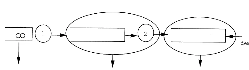
Fig. 1. The two-stage production system.
constraint on the proportion of un"lled demand and give numerical examples.
By quantifying the tradeo!s between single and two parameter policies per stage and single versus two stage control, our comparisons shed further light into the desirable properties and shortcom-ings of a given pull control mechanism.
The outline of the paper is as follows: in Sec-tion 2, we introduce the model and the correspond-ing control problem. We also describe the pull control mechanisms to be analyzed and provide a qualitative comparison based on the control space descriptions of the mechanisms. Single stage control mechanisms di!er from multi-stage mecha-nisms, we describe them brie#y and give a struc-tural result. In Section 3 we give numerical results on the performance of various pull control mecha-nisms and discuss some of the tradeo!s involved. Section 4 studies the extension of the basic model to the case with service level constraints. Our con-clusions are given in Section 5.
2. De5nitions and qualitative results
We consider two single machines in tandem which are connected by an intermediate bu!er. Whenever a part is"nished in the"rst machine, it is placed in an intermediate bu!er and whenever a part is"nished in the second machine, it is placed in the"nished goods inventory. The input bu!er of the"rst machine consists of raw material which is always available, so the"rst machine is never star-ved. The demand that arrives to the system is
satis-"ed from the "nished goods inventory whenever possible and is backlogged otherwise. This system is displayed in Fig. 1. Holding costs are incurred for the parts held in the intermediate bu!er and the
"nished goods inventory. Furthermore, whenever a demand is backordered, backorder costs are in-curred. We are interested in controlling the release of parts from a bu!er to the downstream machine so that the sum of the long-run average holding and backorder costs are minimized.
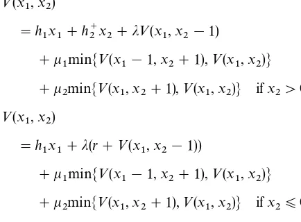
To give a precise description of the model, con-sider the case where demands arrive to the system according to a Poisson process with ratejand the machine in stage i has exponentially distributed service times with ratek
i(i"1, 2). LetX1(t) denote the number of parts in the intermediate bu!er plus the part that is currently in production in the sec-ond machine at timetand letX
2(t) be the number of parts in the"nished goods inventory at time t. Linear holding costs ofh
1proportional toX1(t) is incurred in the"rst stage. As for the second stage, holding costs are incurred at rateh`2 whenever the
"nished goods inventory is non-negative and back-order costs are incurred at rate bwhenever there are backorders. To simplify the notation, we can de"ne the piecewise linear cost function h
2, such that
h
2(x)"
G
h`2x ifx*0,
bx ifx(0. (1)
release policynsuch that the long-run average cost
By standard results in Markov decision pro-cesses, an optimal stationary policyn*exists for the above problem and can be obtained through the solution of the optimality equation:
<(x is the optimal cost per unit time. Note that we have set j#k1#k2"1 without loss of generality as well as using the convention that minM<(x
1,x2), <(x
1!1,x2#1)N"<(x1,x2) whenx1"0.
2.1. Control mechanisms
Below, we introduce the details of the pull type control mechanisms that will be analyzed in the sequel. The development here follows closely that of Liberopoulos and Dallery [7] where more details can be found.
For ease of exposition, we represent all control mechanisms by queueing networks with synchroni-zation stations. All the mechanisms that follow can be represented using at most"ve di!erent type of queues: one corresponding to"nished parts in stage i (denoted by P
i), one corresponding to demands for production of new parts in stagei(D
i), one that corresponds to production authorizations in stage i(A
i), one corresponding to pairs of"nished parts and production authorizations in stagei(PA
i) and the"nal one corresponding to pairs of demands for production and production authorizations in stage i(DA
i). Note thatP0corresponds to the raw parts bu!er which is assumed to be always non-empty. One can also de"ne the queue of parts waiting to be processed in stagei, I
i, for a complete description
although this queue is not critical for our purpose here.
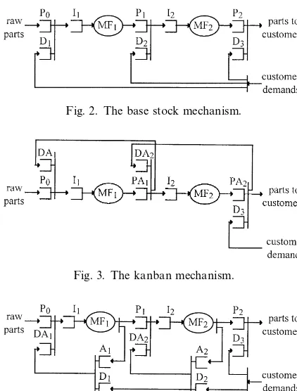
2.1.1. Base stock mechanism
The base stock mechanism is displayed in Fig. 2. In the"gure,D
3corresponds to customer demands. The base stock mechanism is completely described by two parametersS
1andS2corresponding to the base stock levels in stages 1 and 2, respectively. Initially, there are S
1 (S2) parts in queue P1 (P2) while all other queues are empty. Whenever a cus-tomer demand arrives, it joins the queue D
3and requests the release of a"nished part from P
2. At the same time, this demand is also transmitted to D
2 and D1 thereby requesting a release of parts from P
0 to I1 and P1 to I2. Hereon, we use the notation TSBS(S
1,S2) to denote the two stage base stock policy with parametersS
1andS2.
2.1.2. Kanban mechanism
The kanban mechanism can be seen in Fig. 3. Initially, the queue PA
1(PA2) contains K1(K2)
"nished parts each part with a kanban card at-tached on it while all the other queues are empty. Whenever a customer demand arrives to the sys-tem, it joins queueD
3and requests the release of a"nished part from queuePA
2. If a part is avail-able in PA
2, it is released to the customer after having detached the kanban card attached to it. The freed kanban card then joins the queueDA
2 and requests the release of a"nished part fromPA
1 to I
2. If PA1 is not empty, this release will be performed with the kanban detached from the part transferred toDA
1where it will cause the release of a raw part intoI
1. This way, customer demands are transmitted upstream in the system using the kan-ban cards. The control is exerted through the avail-ability of a card in a given stage (if the card is not available at the time of request, demand will not be transmitted upstream until a card becomes avail-able). Once again, the mechanism will be com-pletely described by the initial number of kanban cards at each stage,K
1andK2. We will denote this system by TSK(K
1,K2).
2.1.3. Generalized kanban mechanism
The generalized kanban mechanism [2,3] is displayed in Fig. 4. Initially, the queue P
Fig. 2. The base stock mechanism.
Fig. 3. The kanban mechanism.
Fig. 4. The generalized kanban mechanism.
containsS
1(S2) parts and the queueA1(A2) con-tainsK
1(K2) production authorizations while all other queues are empty. The evolution of gener-alized kanban is very similar to that of the kan-ban mechanism except for the e!ects of the additional (initially) free kanban cards. In the kanban mechanism whenever there are no " nish-ed parts in a certain stage, demand requests cannot be transferred upstream. The additional kanbans in the generalized kanban system serve the pur-pose of relaxing this constraint. In this case, de-mand can be transferred upstream from a stage even in the absence of "nished parts as long as a kanban card is available. We denote the two-stage generalized kanban system with parameters S
1,S2andK1,K2by TSGK(S1,K1,S2,K2). Note that, TSGKS(K
1, K1, K2, K2) is equivalent to TSK(K
1,K2) and TSGK(S1,R,S2,R) is equiva-lent to TSBS(S
1, S2) (see [1,4]).
2.1.4. Extended kanban mechanism
The extended kanban mechanism [4] is dis-played in Fig. 5. In this mechanism, there are
Fig. 5. The extended kanban mechanism.
initiallyS
1(S2) parts with kanbans attached to each of them in queuePA
1(PA2) andK1!S1(K2!S2) free kanbans in queue A
1 (A2) while all other queues are empty. Note that, this mechanism has the condition that K
i*Si(i"1, 2). When a de-mand arrives to the system, it joins the queueD
3as well as the queuesD
2andD1(as in the base stock mechanism). The demand that joins the queue D
3requests a"nished part from queuePA2, if there is a part available in PA
2, it is released to the customer and the detached kanban is transferred to the queue of free kanbans A
2. Concurrently, the demand that has joinedD
2requests the release of a"nished part fromPA
1. The release is now depen-dent on the availability of"nished parts inPA
1as before but also on the availability of free kanbans in the queueA
2. IfPA1andA2are both non-empty, the release takes place, the part from movesPA
1to I
2while a kanban card is transferred fromA2toA1. A similar type of synchronization is required for the release of raw parts fromP
0toA1. We denote the extended kanban system with parameters, S
1, S2andK1,K2by TSEK(S1,K1,S2,K2). As in the generalized kanban system, setting the parameters K
1 and K2 to in"nity in a TSEK results in an equivalence to TSBS(S
1,S2). On the other hand, settingK
i"Si(i"1, 2) in TSEK leads to an equiv-alence to TSK(K
1,K2) (see [1,4]).
2.2. A qualitative comparison: state space repres -entations
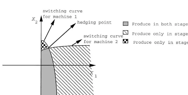
Fig. 6. Optimal switching curves.
regions are separated by monotone switching curves. Fig. 6 displays typical switching curves and the control regions. As can be seen in the "gure, machine 1 is authorized to produce when, x
1, the level of work in process is below a decreasing (inx
2) switching curve. Similarly, machine 2 is authorized to produce when, x
2, the level of "nished goods inventory is below a second (increasing in x
1) switching curve. In fact, note that the regions where only machine 1 or machine 2 is authorized to pro-duce are transient. Monotone control policies can be completely characterized by a pair of switching curves which de"ne the region where both machin-es are authorized to produce. Also note that, the point where the two switching curves intersect is thehedging pointof the system, the point which the control policy drives the system towards. The monotonicity properties provide interesting quali-tative insights into the structure of good control policies. The implications of the monotone struc-ture is quite intuitive; good policies must constrain the work in process levels in addition to the level of
"nished goods inventory. At the same time, the work-in-process levels should change depending on the level of the "nished items bu!er with higher levels of backlog (or lower levels of"nished items) requiring higher (or equivalent) levels of work-in-process. We can qualitatively analyze the
perfor-mance of the pull control mechanisms described earlier keeping these concerns in mind.
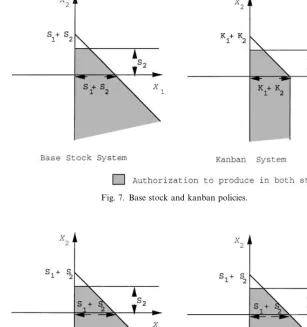
Fig. 7 displays the state space representations of the base stock and kanban policies. Note that, the second stage parametersS
2and K2play identical roles with respect to the control of the second machine. On the other hand, in the base stock mechanism the "rst machine works as long as x
1#x2(S1#S2whereas in the kanban mecha-nism the "rst machine will work as long as x1#x2(K1#K2 and x1(K1#K2. As a result, while the work in process inventoryx
1may grow unboundedly in the base stock mechanism, it is bounded by the total number of production auth-orization cards in the kanban mechanism. In fact, Veatch and Wein [5] prove that the base stock mechanism can never be exactly optimal due to this drawback.
Fig. 8 displays the extended and generalized kanban control mechanisms. The roles of the para-metersS
Fig. 7. Base stock and kanban policies.
Fig. 8. Generalized and extended kanban policies.
slope from!1 toRwhenx2"0, the other two mechanisms have further#exibility in selecting the point where this change occurs. While extended kanban permits changing the slope at levelsx
2)0, generalized kanban permits changing the slope at both positive and negative levels of x
2. In fact, in the particular case of the model considered in this paper, extended kanban can be viewed as a special case of the generalized kanban mechanism. This is an interesting feature of the particular model, since in general both mechanisms have distinctly di!
er-ent behavior and properties as elaborated by Dal-lery and Liberopoulos [4]. The equivalence of the two mechanisms for this model can be explained as follows: although in the TSGK the parameter K
1 does not seem to play a role (see Fig. 8), the de"nition of the mechanism enforces setting K
1*1 as otherwise, the"rst machine would never have the authorization produce. Alternatively, in Fig. 8, initiallyK
1seems to be a crucial parameter but a closer investigation reveals that the selection of K
K
1*S1), since the switching curve (and thus the behaviour) is de"ned by the sum K
1#K2 which can always be adjusted by the choice ofK
2.
2.3. Single-stage control
In the previous sections, we discussed in detail the coordination mechanisms which control the release of material both to the"rst and the second machine. An alternative approach is to view the system as consisting of a single stage which has two machines in tandem and control the release of material only to the "rst machine. In this case, while the "rst machine is directly controlled as before, the second machine is not directly control-led and produces whenever it can (i.e. whenever there are items completed in the "rst stage and waiting to be produced). The single stage kanban system, also known as the CONWIP system (see [6]) has received particular attention. However, single-stage basestock, kanban, generalized kanban mechanisms can also be de"ned analogous to their previously described two stage versions. It turns out that in this case generalized and extended kan-ban policies with identical parameters are equiva-lent [9]. Hence, it will su$ce to consider SSGK from the point of view of performance. We use the shorthands SSBS(S), SSK(K) and SSGK(S,K) to denote these mechanisms having parametersSand K. Our framework enables us to quantify the single stage versus two-stage control tradeo!s through the optimal control framework, but"rst we elabor-ate on some qualitative issues.
Intuitively, the necessity to control the entry of material at multiple stages seems to stem from the fact that as material moves downstream in the production system some value is added to the part in process and as a result the holding costs at upstream stages can be considerably smaller than those at downstream stages. Hence, the di!erence in upstream and downstream holding costs moti-vates keeping inventories upstream whenever pos-sible which implies that it would be necessary to control the release of material in some inter-mediate stages. On the other hand, when hold-ing costs do not change signi"cantly between di!erent stages of the system, it is plausible that
intermediate control points are unnecessary, since in this case what matters is the total number of parts in the system regardless of their particular positions (upstream or downstream). Within our framework, we can concretize this last point by the following proposition which states that whenever holding costs are identical, the optimal policy is to always authorize the machine in the second stage to produce.
Proposition 1. =hen h
1"h`2, the optimal control policy in the second stage is to produce whenever possible(i.e.when x
1*0).
Proof.See the appendix.
Remark 1. Proposition 1 can be interpreted as follows: if holding costs are identical for succesive manufacturing stages, upstream inventories must be transferred to the next stage as fast as possible. It should be noted that some pull control mechanisms violate this proposition by de"nition of their be-havior. This is the case, for instance, of the TSK, for which any positive value ofK
1, parts will be held in queue PA
1 (see Fig. 3) at certain times. On the other hand, in TSBS for example, settingS
1to zero in TSBS(S
1,S2) results in an equivalence with SSBS(S
2). The same equivalence also holds true between TSGK and SSGK, as well as between TSEK and SSEK.
Remark 2.Note that Veatch and Wein [5] provide a proof for the case whenh
1'h`2 using an entirely di!erent approach.
3. Performance analysis
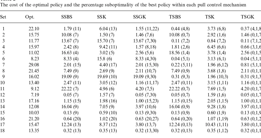
To analyze the performance of control mecha-nisms, we use the following setup. We set the demand ratejto 1 without loss of generality and varyk1andk2as well as the cost parameters. The 18 di!erent sets of data used in the following nu-merical experiments are displayed in Table 1. The
Table 2
The cost of the optimal policy and the percentage suboptimality of the best policy within each pull control mechanism
Set Opt. SSBS SSK SSGK TSBS TSK TSGK
1 22.10 1.79 (11) 6.04 (13) 1.55 (11,22) 0.44 (4,8) 3.73 (6,8) 0.37 (4,1,8,16) 2 15.75 10.08 (7) 1.50 (7) 1.46 (7,6) 10.08 (0,7) 2.92 (1,6) 1.46 (0,1,7,6) 3 11.77 13.67 (7) 15.70 (7) 13.67 (7,30) 0.11 (7,2) 0.84 (7,2) 0.11 (7,1,2,13) 4 15.97 2.42 (8) 9.42 (11) 1.57 (8,18) 1.81 (2,6) 6.45 (6,6) 0.66 (3,1,6,14) 5 11.02 16.63 (4) 3.02 (5) 2.56 (5,6) 18.56 (1,4) 3.78 (1,4) 2.56 (0,1,5,6) 6 8.23 8.33 (4) 15.8 (6) 8.33 (4,30) 0.04 (5,1) 3.13 (6,1) 0.04 (5,1,1,15) 7 29.08 2.01 (15) 4.40 (17) 2.01 (15,30) 0.22 (5,11) 1.96 (6,12) 0.81 (5,1,11,15) 8 21.45 7.49 (9) 2.69 (9) 2.11 (10,7) 7.49 (0,9) 3.68 (1,8) 2.11 (0,1,10,7) 9 16.02 19.09 (9) 19.69 (10) 19.09 (9,30) 0.31 (9,3) 1.96 (10,3) 0.31 (9,1,3,11) 10 13.40 2.47 (11) 3.05 (12) 1.16 (11,17) 2.47 (0,11) 3.15 (1,11) 1.16 (0,1,11,17) 11 9.12 22.22 (7) 4.96 (6) 4.20 (7,5) 22.22 (0,7) 7.69 (1,5) 4.20 (0,1,7,5) 12 7.19 0.05 (7) 1.57 (7) 0.05 (7,30) 0.05 (0,7) 1.59 (1,6) 0.05 (0,1,7,30) 13 17.16 1.15 (15) 1.98 (16) 1.00 (15,23) 1.15 (0,15) 2.05 (1,15) 1.00 (0,1,15,23) 14 12.08 16.04 (9) 7.05 (9) 3.97 (10,6) 16.04 (0,9) 9.28 (1,8) 3.97 (0,1,10,6) 15 10.03 0.13 (9) 0.59 (10) 0.13 (9,30) 0.13 (0,9) 0.60 (1,9) 0.13 (0,1,9,30) 16 21.20 0.64 (20) 1.02 (20) 0.63 (20,27) 0.64 (0,20) 1.07 (1,19) 0.63 (0,1,20,27) 17 15.47 12.24 (13) 8.37 (12) 3.80 (13,7) 12.24 (0,13) 10.43 (1,11) 3.80 (0,1,13,7) 18 13.35 0.32 (13) 0.35 (13) 0.32 (13,30) 0.32 (0,13) 0.35 (1,12) 0.32 (0,1,13,30)
Average suboptimality 7.60 5.96 3.76 5.24 3.59 1.32
Worst-case suboptimality 22.22 19.69 19.09 22.22 10.43 4.2
Table 1
Sets of parameters used Set no k
1 k2 h1 h`2 b
1 1.2 1.2 1 2 4
2 2 1.2 1 2 4
3 1.2 2 1 2 4
4 1.2 1.2 1 2 2
5 2 1.2 1 2 2
6 1.2 2 1 2 2
7 1.2 1.2 1 2 8
8 2 1.2 1 2 8
9 1.2 2 1 2 8
10 1.2 1.2 1 1 2
11 2 1.2 1 1 2
12 1.2 2 1 1 2
13 1.2 1.2 1 1 4
14 2 1.2 1 1 4
15 1.2 2 1 1 4
16 1.2 1.2 1 1 8
17 2 1.2 1 1 8
18 1.2 2 1 1 8
Using the parameter sets in Table 1, we perform the following experiment: for each control mecha-nism of interest, i.e., single-stage base stock (SSBS),
single-stage kanban (SSK), single-stage generalized kanban (SSGK), two-stage base stock (TSBS), two-stage kanban (TSK) and two-stage generalized kanban (TSGK) (we omit extended kanban, since it is a special case of the generalized kanban for this problem), we"nd the values of the parameters that give the minimum cost by performing a search in the state space combined with the value iteration algorithm (see [10] for example). We also compute the optimal policy for the given parameters by using value iteration in a truncated state space (state spaces of dimension up to 50 by 100 have been used). The comparisons are hence between the best performances that can be obtained from a given mechanism. In Table 2, we report the cost achieved by the optimal policy (denoted by`Opt.a in the table) and the percentage suboptimality of the minimum cost achieved by each mechanism as well as the parameters of each mechanism yielding the minimum cost (given in parenthesis after the suboptimality value). The parameters are given in the order de"ned in the previous sections. In dis-playing the parameters, we set K
Consider the columns of Table 2, that corres-pond to single-stage control mechanisms. We observe in general that in most cases, either SSBS or SSK performs well. A more careful observa-tion reveals that for the cases where both machines have equal production rates (data sets 1, 4, 7, 10, 13 and 16) SSBS performs better than SSK and for the cases where the second mac-hine is slower than the"rst machine (data sets 2, 5, 8, 11, 14 and 17) SSK performs better. In either case (when data sets 3, 6, 9, 12, 15 and 18 are excluded), SSGK is the clear winner with a maximum error of 4.2%. One would be tempted to state that single stage policies are extremely e$cient if it were not for the less than satis-factory results obtained in data sets 3, 6 and 9. The common characteristics of these sets are a fas-ter production rate in the second machine and higher holding costs in stage 2 than stage 1. The imbalance between the machines necessitates a considerable amount of safety stock in between but since holding "nished goods inventory is expensive, this safety stock should not be converted into "nished goods until necessary and this can only be achieved by controlling the machine in the second stage.
The columns of Table 2 corresponding to two stage policies reveal other interesting properties. Firstly, TSBS performs better than TSK in all cases except those where the "rst machine is faster than the second machine. The problem, however, is that when TSBS performs worse that TSK, it performs poorly whereas TSK seems more robust. In any case, when robustness is the issue TSGK is con-siderably more reliable than either TSK or TSBS. Once again, the interesting observation here is that usually either TSK or TSBS performs well while TSGK always performs well since it can imitate the better system by an appropriate choice of the para-meters.
Finally, note that in rows corresponding to para-meter sets 10}18 of Table 2 SSKS performs better than TSKS while SSBS and SSGK perform as well as TSBS and TSGK respectively. This is not sur-prising in light of our previous results since this part of the data set corresponds to the the cases where the holding costs are identical in both stages of the system.
4. Service level constraints
It is frequently argued that although backorder-ing demand is an important concern, backlog costs are di$cult to quantify. An alternative approach to analyze the tradeo! due to un"lled demand is through service level constraints. A frequently used service level is,ll ratede"ned as the proportion of demands that can be satis"ed from on hand inven-tory upon arrival. In this section, we extend the previous discussion on qualitative properties of good control policies to systems with "ll rate constraints.
Consider a "ll rate constraint of the following type: the probability of ful"lling an order from on hand inventory upon arrival must be at least
(1!a). To make this de"nition more precise, let
t
nbe the time corresponding to thenth event (arri-val of demand or service completion in either stage) in the system. Let I
A( ) be the indicator function that corresponds to the demand arrival event, i.e., I
A(tn)"1 if thenth event is an arrival andIA(tn)"0 otherwise. Furthermore, we can de"ne a second indicator function,I
b( ) that marks demand arrivals that are not satis"ed from on-hand inventory. Hence,
The"ll rate constraint is then
lim
In other words, by setting the backorder cost b"0, we obtain the identical objective function as in Eq. (2), however this time the minimization is subject to the constraint Eq. (4).
constraint to the objective function with a penalty of r. The resulting problem is referred to as the problem with un,ll penalties.
To analyze the problem with un"ll penalties, note that the Lagrangian leads to the following optimality equations:
once again with the convention that minM<(x 1!1, x
2#1),<(x1,x2)N automatically equals <(x1,x2) wheneverx
1"0.
Examining the above optimality equations, we note that the un"ll penalties can be converted into equivalent backorder costs. The equivalent backor-der cost function is given by
h
2(x)"
G
h`2x ifx'0,
jr ifx)0. (6)
The only di!erence between the backorder cost and un"ll penalty problems is the backorder cost function. This prompts the question as to whether the monotonicity properties are retained for this problem as well. Unfortunately, the new holding cost function does not satisfy the directional sub-modularity conditions used by Veatch and Wein [8] to prove monotonicity which rules out an inductive proof. Furthermore, there are numerical examples in which optimal switching curves are not monotone. Nevertheless, in most numerical examples the optimal switching curves seem to be monotone.
To relate the problem with un"ll penalties to the one with service level constraints, note that each un"ll penalty rinduces an associated"ll ratea(r).
One can then varyruntila(r) is su$ciently close to the desired service levela. The optimal holding cost under this policy can then be computed by"xing the policy and recomputing the cost by setting r"0.
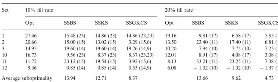
Table 3 reports the optimal performance of single stage base stock, kanban and generalized kanban policies for di!erent parameter sets under two di!erent "ll rate constraints, 10% and 20%. The`Opt.acolumn reports the results of the min-imum cost found by the Lagrangian heuristic (which is not necessarily the minimum cost that can be obtained by a stationary policy, in fact in the last row of the table the all three control mechanisms perform better than the Lagrangean heuristic.).
Table 3 is consistent with the preceding numer-ical results on the case with linear backorder costs. The SSGK performs signi"cantly better than SSBS and SSK on the average. Furthermore, the di!erence in the average performance is sharp-ened due to the existence of cases where single parameter policies can perform quite poorly (such as the case in the rows corresponding to parameter sets 2 and 11).
5. Conclusion and future research
Using a two stage model and an optimal control approach, we presented performance comparisons between various control mechanisms. It turns out that simple mechanisms such as kanban, base stock and even their single-stage variants are very e! ec-tive for the model considered. On the other hand, these simple mechanisms have a major drawback in that under certain conditions they can perform poorly. This highlights the signi"cant advantage of more complicated mechanisms such as generalized or extended kanban. These mechanisms do not necessarily perform signi"cantly better than simpler ones for a given case but they are guaran-teed to perform well under all circumstances.
Table 3
Service level constraint results
Set 10%"ll rate 20%"ll rate
Opt SSBS SSKS SSGKCS Opt SSBS SSKS SSGKCS
1 27.46 15.48 (23) 14.86 (23) 14.86 (23,23) 19.16 9.81 (17) 6.58 (17) 5.85 (17,16) 2 20.66 15.00 (15) 13.02 (15) 3.29 (15,6) 13.50 23.40 (11) 17.40 (11) 6.81 (11,6) 3 14.95 19.60 (14) 19.60 (14) 19.26 (14,9) 10.20 7.94 (10) 7.75 (10) 7.25 (10,8) 10 16.73 9.56 (23) 8.37 (23) 8.37 (23,23) 12.01 8.91 (17) 4.08 (17) 3.08 (17,16) 11 11.72 23.12 (15) 19.54 (15) 3.92 (15,6) 8.13 33.21 (11) 23.25 (11) 7.38 (11,6) 12 9.36 0.85 (14) 0.85 (14) 0.53 (14,9) 6.08 !1.32 (10) !1.32 (10) !1.97 (10,8)
Average suboptimality 13.94 12.71 8.37 13.66 9.62 4.73
Worst-case suboptimality 23.12 19.60 19.26 33.21 23.25 7.38
could be useful from the design point of view is that good generalized (or extended) kanban policies in general tend to imitate the better of base stock and kanban policies. It seems plausible then to consider an approach where a good base stock or kanban policy is improved upon by iteratively adjusting the additional parameters to obtain a good generalized or extended kanban policy.
Another interesting and relevant extension is to consider multiple part types. This brings in the additional di$culty of sharing manufacturing resources between di!erent part types in addition to the decisions of whether or not to produce that were considered for the single part type case. The design of simple but e!ective multistage pull mech-anisms for multiple part type systems remains as a challenging issue for future research.
Appendix A.
Proof of Proposition 1. Consider the case of min-imizing the total discounted costs over an in"nite horizon with discount factora, i.e., we would like to
"nd the policy that minimizes
lim T?=
supE
C
TP
0 e~at(h
1X1(t)#h2(X2(t))) dt
D
. (A.1)Let j#k1#k2#a"1 without loss of general-ity, the corresponding optimality equations are as
follows:
<(x 1,x2)
"h
1(x1)#h2(x2)#j<(x1,x2!1)
#k1minM<(x
1#1,x2),<(x1,x2)N
#k2minM<(x
1!1,x2#1),<(x1,x2)N. (A.2)
We would like to argue through value iteration by using the fact that the optimal in"nite horizon cost<(x
1,x2) can be obtained as the limit of corre-sponding k-horizon cost functions as the hor-izonk tends to in"nity. To this end let<k(x
1,x2) denote the the minimum total cost incurred over kstages starting from state (x
1,x2). Furthermore, let<0(x
1,x2)"0 for allx1andx2.
To obtain the necessary result, we need to show that
minM<(x
1!1,x2#1),<(x1,x2)N
"<(x
1!1,x2#1) (A.3)
or equivalently<(x
1!1,x2#1))<(x1,x2), when-everx
1'0.
The above property holds trivially for<0(x 1,x2), now we assume that it also holds true for<k(x
<k`1(x Now we will perform a term by term comparison:
"rstly, since h
1"h`2,h1(x1!1)#h2(x2#1)) h
1x1#h2(x2). Secondly, j<k(x1!1,x2))j<k(x1, x
2!1) by the induction assumption. By the same assumption: k2<k(x
1!2,x2#2))k2<k(x1!1, x
2#1). Hence, we are left with the terms corre-sponding to production in the"rst stage. We con-centrate on these terms by considering all four possible combinations of control actions:
Case1: Optimalkth stage actions are to produce in stage 1 in both (x
1,x2) and (x1!1,x2#1). In this case, the resulting term on the right-hand side of (A.4) is<k(x
1#1,x2) and the term on the right-hand side of (A.5) is: <k(x
1,x2#1). By the in-duction assumption, we have: <k(x
1,x2#1)) <k(x
1#1,x2).
Case 2: Optimal kth stage actions are not to produce in machine 1 in both (x
1,x2) and (x
1!1,x2#1). The desired inequality is obtained exactly as in the previous case by the induction assumption.
Case 3: Optimal kth stage actions for machine 1 are to produce in state (x
1,x2) and not produce in state (x
1!1,x2#1). This case can not happen since it contradicts the monotonicity property pro-ved in Veatch and Wein [8] which states that if it is optimal to produce in machine 1 in state (x1,x2), it
is also optimal to produce in machine 1 is state (x
1!1,x2#1).
Case4: Optimal kth stage actions for machine 1 are not to produce in state (x
1,x2) by the induction assumption giving the desired inequality.
We have proved that the desired property propa-gates through value iteration. To complete the proof, we note that the in"nite horizon problem will also inherit the desired property by letting kPR. Furthermore, under standard assump-tions, limits can be taken as the discounting factor aapproaches 1 to show that average cost per unit time problem also has the identical property.
References
[1] J.A. Buzacott, J.G. Shanthikumar, Stochastic Models of Manufacturing Systems, Prentice-Hall, New York, 1993. [2] J.A. Buzacott, Queueing models of kanban and MRP
controlled manufacturing systems, Engineering Cost and Production Economics 17 (1989) 3}20.
[3] P. Zipkin, A Kanban like production control system: Analy-sis of simple models, Research Working Paper No. 89-1, Graduate School of Business, Columbia University, New York, 1989.
[4] Y. Dallery, G. Liberopoulos, Extended kanban control system: A new kanban type pull control mechanism for multi-stage manufacturing systems, Working Paper, 1997. [5] M.H. Veatch, L.M. Wein, Optimal control of a make-to-stock production system, Operations Research 42 (1994) 337}350.
[6] M.L. Spearman, D.L. Woodru!, W.J. Hopp, CONWIP: a pull alternative to kanban, International Journal of Pro-duction Research 28 (1990) 879}894.
[7] G. Liberopoulos, Y. Dallery, A uni"ed framework for pull control mechanisms in multi stage manufacturing systems, Working Paper, 1997.
[8] M.H. Veatch, L.M. Wein, Monotone control of queueing networks, Queueing Systems 12 (1992) 391}408. [9] G. Liberopoulos, Y. Dallery, On the optimization of single
stage kanban-type control systems in manufacturing, Working Paper, 1995.