Directory UMM :Data Elmu:jurnal:J-a:Journal of Econometrics:Vol95.Issue1.2000:

*Tel.: 042-580-8367; fax: 042-580-8333.

E-mail address:cr00387@srv.cc.hit-u.ac.jp (T. Nakatsuma)

Bayesian analysis of ARMA}GARCH models:

A Markov chain sampling approach

Teruo Nakatsuma

*

Institute of Economic Research, Hitotsubashi University, Naka 2-1, Kunitachi, Tokyo, 186-8603, Japan

Received 1 August 1996; received in revised form 1 February 1999; accepted 1 April 1999

Abstract

We develop a Markov chain Monte Carlo method for a linear regression model with

an ARMA(p,q)-GARCH(r,s) error. To generate a Monte Carlo sample from the joint

posterior distribution, we employ a Markov chain sampling with the Metropolis}Hastings algorithm. As illustration, we estimate an ARMA}GARCH model of simulated time series data. ( 2000 Elsevier Science S.A. All rights reserved.

JEL classixcation: C11; C22

Keywords: ARMA process; Bayesian inference; GARCH; Markov chain Monte Carlo; Metropolis}Hastings algorithm

1. Introduction

In this paper, we propose a new Markov chain Monte Carlo (MCMC) method for Bayesian estimation and inference of the ARCH/GARCH model. Autoregressive conditional heteroskedasticity (ARCH) by Engle (1982) and generalized ARCH (GARCH) by Bollerslev (1986) have been extensively studied and applied in many"elds of economics, especially in"nancial economics. Our

1Importance sampling, another popular Monte Carlo integration method, was also applied to ARCH and GARCH models by a few researchers (Geweke, 1989a, b; Kleibergen and Van Dijk, 1993, among others).

new MCMC method is applicable to estimating not only a simple ARCH/ GARCH model but also a linear regression model with the ARMA}GARCH error, which we shall call the ARMA}GARCH model.

The MCMC method is one of Monte Carlo integration methods.1 In this method, we generate samples of parameters in the model from their joint posterior distribution by Markov chain sampling, and evaluate complicated multiple integrals, which are necessary for Bayesian inference, by Monte Carlo integration. The Metropolis}Hastings (MH) algorithm is one of the Markov chain sampling schemes widely used among researchers. The MH algorithm, developed by Metropolis et al. (1953) and Hastings (1970), is a technique to generate random numbers from a probability distribution. This algorithm is quite useful especially when we cannot generate samples of the parameters directly from their joint posterior distribution. This is the case for the ARMA}GARCH model.

To develop a new MCMC method for the ARMA}GARCH model, we combine and modify Markov chain sampling schemes developed by Chib and Greenberg (1994) and MuKller and Pole (1995). Chib and Greenberg (1994) designed a Markov chain sampling scheme for a linear regression model with an ARMA(p,q) error in which the disturbance term of the ARMA process was i.i.d. normal. MuKller and Pole (1995) developed an MCMC procedure for a linear regression model with a GARCH error in which the error term of the regression model had no serial correlation. It seems natural to develop a new MCMC procedure for the ARMA}GARCH model by combining these two methods.

Organization of this paper is as follows. In Section 2, we explain our new MCMC method for the ARMA}GARCH model. In Section 3, we estimate ARMA}GARCH models with simulated data by our MCMC method as illus-tration. In Section 4, concluding remarks of this paper are given.

2. MCMC method for ARMA}GARCH models

2.1. ARMA}GARCH model and Bayesian inference

We consider the following linear regression model with an ARMA(p,q)}GARCH(r, s) error, or simply an ARMA}GARCH model:

y

u independent variables;cis ak]1 vector of the regression coe$cients;F

t~1is

In practice, we often impose several constraints on parameters in the ARMA}GARCH model:

C1 and C2 are related to stationarity and invertibility of the ARMA process. C3 and C4 are imposed to guarantee that the conditional variancep2

t is always positive. In many previous studies of GARCH models, the following constraint:

C5:A(1)#B(1)(1,

is imposed for the"niteness of the unconditional variance ofe_t. Since one of the objects in Bayesian analysis of the ARMA}GARCH model is to test whether the constraint C5 is true, we will not put C5 on the GARCH coe$cients.

To perform Bayesian analyses of the ARMA}GARCH model, we construct the posterior density function of the model:

p(dD>_,X)" l(

>_{DX, d)p(d)}

:l₍>_{DX,d)p(d) dd}, (3)

wheredis the set of all parameters in the ARMA}GARCH model,l₍>_{DX,d) is}

the likelihood function, and p(d) is the prior. The likelihood function of the ARMA}GARCH model is

and we assume y

0"e0, yt"0 for t(0, and xt"0 for t)0. We treat the pre-sample errore₀as a parameter in the ARMA}GARCH model.

As the prior, we use the following proper prior:

p(e₀,c,/,h,a,b)"N(k_e

0,Re0)]N(kc,Rc) ]N(k₍,R

()IC1(/)]N(kh,Rh)IC2(h)

]N(k_a,R

a)IC3(a)]N(kb,Rb)IC4(b), (6)

where I

Cj())(j"1, 2, 3, 4) is the indicator function which takes unity if the constraint holds; otherwise zero, and N())I

Cj()) represents that the normal distribution N()) is truncated at the boundary of the support of the indicator functionI

Cj()).

In Bayesian inference, we need to evaluate the expectation of a function of parameters:

E[f(d)]"

P

f(d)p(dD>_{, X) dd. (7)}

The functional form off(d_j) depends on what kind of inference we conduct. For instance, when we estimate the posterior probability ofA(1)#B(1)(1,f(d) is the indicator functionI(A(1)#B(1)(1).

In the ARMA}GARCH model (1) and (2), however, it is di$cult to evaluate the multiple integral in (7) analytically. We need to employ a numerical integra-tion method. A Monte Carlo integraintegra-tion is one of widely used techniques for numerical integration. LetMd(1),2, d(m)Nbe samples generated from the

poste-rior distributionp(dD>_{,X). Then (7) is approximated by}

E[f(d)]+1

m m

+

i/1

f(d(i)) (8)

for enough largem.

To apply the Monte Carlo method, we need to generate samples

Md(1),2, d(m)Nfrom the posterior distribution. Since we cannot generate them

directly, we use the Metropolis}Hastings (MH) algorithm, which is one of Markov chain sampling procedures such as the Gibbs sampler. In the MH algorithm we generate a valuedK from the proposal distributiong(d) and accept the proposal value with probability:

j(d, dK)"min

G

p(dKD>, X)/g(dK)

p(dD>_,X)/g(d), 1

H

. (9)

2You may suspect that this normal approximation is quite poor, but in our experience this approach works"ne.

2.2. MCMC procedure

We explain the outline of our new MCMC procedure for the ARMA}

GARCH model. More details on the MCMC procedure are given in the appendix of this paper.

To construct a MCMC procedure for the ARMA}GARCH model, we divide the parameters into two groups. Let d₁"(e₀,c, /,h) be the "rst group and

d₂"(a, b) be the second. For each group of the parameters, we use di!erent proposal distributions.

The proposal distributions for the "rst groupd₁are based on the original ARMA}GARCH model: but we assume that the conditional variances Mp2_tN_nt/1 are "xed and known. Using (10), we can generated₁from their proposal distributions by the MCMC procedure by Chib and Greenberg (1994) with some modi"cations.

The proposal distributions for the second groupd₂are based on an approxi-mated GARCH model: by using the well-known property of the GARCH model. As shown in Bollerslev (1986), the GARCH(r, s) model (2) is expressed as an ARMA(l, s) process of

t~1)"0, and the conditional variance is

Var(w8_tDF

t~1)"2p4t. Replacing w8t with wt&N(0, 2p4t)2, we have (11). Given

Mp2

tNnt/1and Me2tNnt/1, we generate d2from their proposal distributions by the

MCMC procedure similar to Chib and Greenberg's method.

The outline of our MCMC procedure is as follows:

(b) generated₂"(a, b) from the proposal distribution based on (11) givend₁, (c) apply the MH algorithm after each parameter is generated in (a) or (b), (d) repeat (a)}(c) until the sequences become stable.

In this procedure, we updateMe2_tN_nt/1andMp2_tN_nt/1at every time after correspond-ing parameters are updated. The full description of our new procedure is given in the appendix of this paper.

3. An example of the MCMC estimation

In this section, we demonstrate how our new MCMC method is used in application. We consider the following regression model:

y

t"c1#c2xt#ut, (t"1,2, n) u

t"/1ut~j#et#h1et~1#h2et~2#h3et~3#h4et~4,

e_tDF

t~1&N(0,p2t),

p2_t"_a

0#a1e2t~1#a2e2t~2#a3e2t~3#a4e2t~4#b1p2t~1

#_b

2p2t~2,

(13)

where

(c₁,c₂)"(1.0, 1.0),

/₁"0.9,

(h₁, h₂, h₃, h₄)"(!0.48, 0.36,!0.24, 0.12), (a₀, a₁, a₂, a₃,a₄)"(0.001, 0.24, 0.18, 0.12, 0.06), (b₁, b₂)"(0.2, 0.1),

x

t is drawn from the uniform distribution between!0.5 and 0.5, and we set n"1000.

We estimate (13) by our new MCMC method and the maximum-likelihood estimation (MLE) for comparison. The maximum-likelihood estimates of the parameters are computed with the simulated annealing algorithm by Go!e (1996). For this data set, the covariance estimatorn~1A~1₀ B

0A~10 , where

A₀"!1

n n

+

t/1

A

R_2lnl

t(d)

R_dR_d@

B

and B0" 1 n

n

+

t/1

A

R_lnl

t(d) R_d

R_lnl t(d) R_d@

B

,

is not positive de"nite at the maximum-likelihood estimates ofdbecauseA 0is

not. Therefore, we usen~1B~1₀ as the covariance estimator.

3We also tried to use every third,"fth or tenth point, instead of all points, in the sample path to avoid strong serial correlation. The changes in estimation results, however, were negligible.

discarded as the initial burn-in is determined by the convergence diagnostic (CD) in Geweke (1992). Letm

0denote the number of runs to be discarded, and mthe number of runs to be retained. LetdM₁denote the sample mean ofdfor the

"rstm

1runs in the sample path withm runs, anddM2for the last m2runs. As

Geweke (1992) suggested, We setm

1"0.1 m andm2"0.5 m. The test statistic

for CD is given as

(dM₁!_dM

2)/[SKd1(0)/m1#SKd2(0)/m2]1@2, (14)

whereSKd

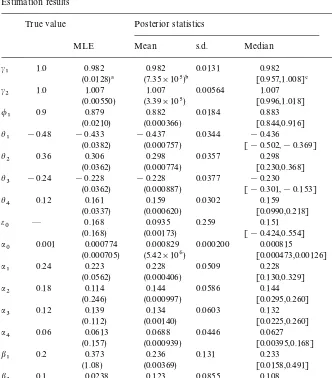
i()) is the spectrum density estimate formiruns, and (14) asymptotically follows the standard normal distribution. By this diagnostic, we choose m₀"6000 and m"54,000.3Estimation results by the MLE and the MCMC are shown in Table 1.

In Table 1, the MLE and the MCMC produce comparable estimates forc,/, andh. Allt-ratios of these parameters in the MLE are greater than 2.0. Foraand

b, however, thet-ratios are less than 2.0 except fora₁. In the MCMC, the 95% interval does not include zero forc, /, andh(this fact is guaranteed foraand

b by assumption), and the true value is within the 95% interval for all para-meters.

We also estimate the posterior probability of A(1)#B(1)(1, the condition for the "nite unconditional variance in the GARCH(p,q) process (2). This probability is estimated by (8) with f(d)"I(A(1)#B(1)(1). The estimated posterior probability is shown in the bottom of Table 1. The value, 0.917, is reasonable because A(1)#B(1)"0.24#0.18#0.12#0.06#0.2#0.1"

0.9(1 and the GARCH process in (13) has the"nite unconditional variance.

4. Concluding remarks

In this paper, we derived a Markov chain Monte Carlo method with Metrop-olis}Hastings algorithm for Bayesian inference of a linear regression model with an ARMA}GARCH error,or the ARMA}GARCH model. Our new MCMC method allows the error term not only to be an ARMA(p,q) process, but also to have the GARCH variance. This#exibility is one of the major advantages of our new method. Moreover, our method can deal with the pre-sample values of the error term and conditional variance of the ARMA}GARCH model.

Table 1

Estimation results

True value Posterior statistics o($

MLE Mean s.d. Median CD%

c₁ 1.0 0.982 0.982 0.0131 0.982 0.143

(0.0128)! (7.35]105)" [0.957,1.008]# !0.551

c₂ 1.0 1.007 1.007 0.00564 1.007 0.168

(0.00550) (3.39]105) [0.996,1.018] !0.435

/

1 0.9 0.879 0.882 0.0184 0.883 0.706

(0.0210) (0.000366) [0.844,0.916] 0.209

h₁ !0.48 !0.433 !0.437 0.0344 !0.436 0.908

(0.0382) (0.000757) [!0.502,!0.369] 1.43

h₂ 0.36 0.306 0.298 0.0357 0.298 0.903

(0.0362) (0.000774) [0.230,0.368] !0.756

h₃ !0.24 !0.228 !0.228 0.0377 !0.230 0.911

(0.0362) (0.000887) [!0.301,!0.153] !0.0146

h₄ 0.12 0.161 0.159 0.0302 0.159 0.893

(0.0337) (0.000620) [0.0990,0.218] 0.600

e₀ * 0.168 0.0935 0.259 0.151 0.373

(0.168) (0.00173) [!0.424,0.554] 0.0750

a₀ 0.001 0.000774 0.000829 0.000200 0.000815 0.691

(0.000705) (5.42]106) [0.000473,0.00126] !0.502

a₁ 0.24 0.223 0.228 0.0509 0.228 0.406

(0.0562) (0.000406) [0.130,0.329] 0.507

a₂ 0.18 0.114 0.144 0.0586 0.144 0.546

(0.246) (0.000997) [0.0295,0.260] !0.660

a₃ 0.12 0.139 0.134 0.0603 0.132 0.604

(0.112) (0.00140) [0.0225,0.260] 0.276

a₄ 0.06 0.0613 0.0688 0.0446 0.0627 0.566

(0.157) (0.000939) [0.00395,0.168] !0.746

b₁ 0.2 0.373 0.236 0.131 0.233 0.805

(1.08) (0.00369) [0.0158,0.491] !0.100

b₂ 0.1 0.0238 0.123 0.0855 0.108 0.624

(0.559) (0.000927) [0.00558,0.314] 1.17

PMA(1)#B(1)(1N 0.917 0.275 * 0.249

(0.00165) 0.700

!the standard error of the MLE.

"the numerical standard error of the posterior mean.

#95% interval, [Q

2.5{,Q_97.5{].

$the"rst-order autocorrelation in a sample path.

%convergence diagnostic test statistic (14).

chain sampling. We estimated the posterior statistics of the parameters and compare them to the MLE. We also estimated the posterior probability of the

Appendix A

In this Appendix, we explain the proposal distributions of parameters in the ARMA}GARCH model for the MCMC procedure. The parameters to be generated are (i) pre-sample error e₀; (ii) regression coe$cients c; (iii) AR coe$cients /; (iv) MA coe$cients h; (v) ARCH coe$cients a; (vi) GARCH coe$cients b. We also discuss how to deal with the pre-sample error of the approximated GARCH model (11),w

0.

A.1. e₀:Pre-sample error

Given the pre-sample errore₀, the ARMA}GARCH model is rewritten as

y

derived a similar expression for a regression model with an ARMA(p, q) error. The likelihood function of the ARMA}GARCH model is rewritten as

f(>_{DX, R, d}

We have the proposal distribution ofe₀:

e₀D>_,X,R&N(k(_e

0,p(e0), (A.4)

wherek(

e0"RKe0(+nt/1x2et/p2t#ke0/p2e0) andRKe0"(+nt/1xetyet/p2t#p~2e0 )~1. A.2. c:Regression coezcients

The likelihood function of the ARMA}GARCH model is rewritten as

whereyH_t andxH_t are calculated by the following transformation:

"ed version of the transformation derived by Chib and Greenberg (1994). It is straightforward to show e

t"yHt!xHtc. Let >c"[yH1,2,yHn]@ and X_c"[xH₁{,2,xH{

n]@. We have the following proposal distribution of c:

cD>_{, X, R,d}

~c&N(k(c, RKc), (A.7) wherek(_c"RK_c(X@_cR~1>

c#R~1c kc) andRKc"(X@cR~1Xc#R~1c )~1.

A.3. /:AR coezcients

The likelihood function of the ARMA}GARCH model is also written as

f(>_{DX, R, d}

wherey8_t andx8_tare calculated by the following transformation:

y8 transformation derived by Chib and Greenberg (1994). It is also straightforward to showe

t"y8t!x8t/. Let>("[y81,2, y8n]@andX("[x8 @1,2, x8 @n]@. We have the proposal distribution of/:

/D>_{,X, R, d}

~(&N(k((, RK()IC1(/), (A.10)

wherek(

("RK((X@(R~1>(#R~1( k() andRK("(X@(R~1X(#R~1( )~1.

A.4. h:MA coezcients

Generation of h is a little more complicated since the error term u t is a non-linear function ofh. To deal with this complexity, Chib and Greenberg (1994) proposed to linearizee_tby the"rst-order Taylor expansion

e_t(h)+_e

wheree_t(hH)"yH_t(hH)!xH_t(hH) andt_t"[t_1t,2,t_qt] is the "rst-order

deriva-tive ofe_t(h) evaluated athHgiven by the following recursion:

t_it"!_e mation. Chib and Greenberg (1994) chose the non-linear least-squares estimate ofhgiven the other parameters ashH,

hH"argmin

However, the error term in the ARMA}GARCH model is heteroskedastic while Chib and Greenberg applied their approximation to the homoskedastic-error ARMA model. Thus, instead of (A.13), we use the following weighted non-linear least-squares estimate ofh:

hH"argmin

to approximate the likelihood function for model (10).

Then we have an approximated likelihood function for model (10):

f(>_{DX, R, d} approximated likelihood function, we have the following proposal distribution ofh:

0:Pre-sample error in the approximated GARCH model

Before we explain the proposal distributions foraandb, we discuss how to deal with the pre-sample error in the approximated GARCH model (11),w

Unlikee₀, we do not need to generatew

0. Suppose that the initial variance p2₀is equal toa₀. Sincew

t"e2t!p2t, we have w

0"e20!a0. (A.18)

Hence,w₀is automatically determined by (A.18) once we obtaine₀anda₀.

A.6. a:ARCH coezcients

Generation ofais similar to/. The likelihood function of the approximated GARCH model (11) is rewritten as

f(e2D>_{, X, R, d}

A.7. b: GARCH coezcients

Generation of bis similar toh. We approximate the likelihood function of (11) as which is computed by the transformation (A.12) with!_e

t~i(hH)Pp2t~i(bH) and

hH

jP!bHj, and bH is the solution of (A.14) with hPb, et(h)Pwt(b), and

p2_tP2p4_t. Let>

b"[w1(bH)#m1bH,2,wn(bH)#mnbH]@andXb"[m@1,2,m@n]@. Using the approximated likelihood function (A.21), we have the following proposal distribution ofb:

bD>_{,X,R, d}

~b&N(k(b, RKb)IC4(b), (A.22)

wherek(

References

Bollerslev, T., 1986. Generalized autoregressive conditional heteroskedasticity. Journal of Econo-metrics 31, 307}327.

Chib, S., Greenberg, E., 1994. Bayes inference in regression models with ARMA (p,q) errors. Journal of Econometrics 64, 183}206.

Chib, S., Greenberg, E., 1995. Understanding the Metropolis}Hastings algorithm. American Statisti-cian 49, 327}335.

Engle, R.F., 1982. Autoregressive conditional heteroskedasticity with estimates of the variance of United Kingdom in#ation. Econometrica 50, 987}1008.

Geweke, J., 1989a. Bayesian inference in econometric models using Monte Carlo integration. Econometrica 57, 1317}1339.

Geweke, J., 1989b. Exact predictive densities for linear models with ARCH disturbances. Journal of Econometrics 40, 63}86.

Geweke, J., 1992. Evaluating the accuracy of sampling-based approaches to the calculation of posterior moments. In: Bernardo, J.M., Berger, J.O., Dawid, A.P., Smith, A.F.M. (Eds.), Bayesian Statistics 4. Oxford University Press, Oxford, pp. 169}193.

Go!e, W.L., 1996. SIMANN: a global optimization algorithm using simulated annealing. Studies in Nonlinear Dynamics and Econometrics 1, 169}176.

Hastings, W.K., 1970. Monte Carlo sampling methods using Markov chains and their applications. Biometrika 57, 97}109.

Kleibergen, F., Van Dijk, H.K., 1993. Non-stationarity in GARCH models: A Bayesian analysis. Journal of Applied Econometrics 8, S41}S61.

Metropolis, N., Rosenbluth, A.W., Rosenbluth, M.N., Teller, A.H., Teller, E., 1953. Equations of state calculations by fast computing machines. Journal of Chemical Physics 21, 1087}1092. MuKller, P., Pole, A., 1995. Monte Carlo posterior integration in GARCH models. Manuscript, Duke

University.