A C
OMPARATİVE
EARTHWORK AND COST A
NALYSİS OF
IMPROVING AN
E
XİSTİNG
R
AİLWAY
L
İNE AND
CONSTRUCTING A NEW HIGH-SPEED LINE IN
TURKEY
K. A. Gumusa, V. E. Gulalb
a Turkish State Railways, Department of Survey, Project and Investment, 06330 Altındag, Ankara, Turkey - [email protected]
b Yildiz Technical University, Department of Geomatics Engineering, 34220 Davutpasa, Istanbul, Turkey - [email protected]
KEY WORDS: High-Speed Railways, High-Speed Track, Track Geometry, Track Design, Cost Analysis
ABSTRACT:
In the past few decades, high-speed railways have become an important transportation system due to their high operational speed, and globally, the networks of these railways have been extended. In addition, there is ongoing work on the construction of new high-speed railways as well as improving existing lines to achieve the same operational speed. To contribute to high-speed railway works in Turkey, this study compared two high-speed railway lines; an existing conventional line, the design of which was improved, and a new high-speed line. The design of an existing conventional railway line was improved according to optimal geometric characteristics of high-speed railways and an alternative line was simulated. These two lines were evaluated on three different types of land in terms of the required volume of earthworks, engineering structures and total cost. The results show that the length of the conventional line was reduced after the improvement process; however, new engineering structures are needed. Furthermore, compared to the alternative line, the track length and total length of engineering structures required for the improvement of the existing line was shorter and the volume of required earthworks was less resulting in lower costs.
1. INTRODUCTION
As with other transportation systems, railways consist of multiple elements including the route network, vehicle fleet and the operation system (Yalçın, 2007). There are two types of railways; high-speed and conventional. According to the directive 94/48/EC of the Council of the European Union, the term ‘high-speed’ covers all railway express services operating at speeds within the 200 to 300 km/h range (Mundrey, 2010) and railways operating at a speed below this range are considered conventional. Due to their different requirements in terms of speed, the geometric specifications, infrastructure and superstructure of high-speed and conventional railways differ (Ekim, 2010). After the work on high-speed railways began in Japan in 1964, there has been a rapid expansion of high-speed railway networks, particularly in Europe and Asia (Esveld, 2010).
In Turkey, the construction and development of high-speed railways gained more importance and speed after 2000. This study aimed to contribute to high-speed railway works in Turkey by comparing two high-speed railway lines; an existing conventional line, the design of which was improved, and an alternative line.
In the literature, there are several studies on the geometric characteristics and design of railway lines. In this study, the design parameters for the improvement of the existing line and simulation of the alternative were based on previous work by two researchers. The first is Lindahl (2001), who compared the geometric characteristics of high-speed railways used in the world and a simulated line. Based on the results, the author suggested new limits regarding the geometric characteristics of high-speed railways. The second is Hodas (2014), who created three designs for high-speed railway lines using 3D modeling software in accordance with the standards provided by the European Committee for Standardization (CEN), the newly prepared and current geometric standards for the Slovak
Railways, and compared the designs with each other. The author concluded that the design work entails complicated procedures with the design of both slow- and high-speed railway lines being equally difficult. However, Hodas added that these two types of lines have different design parameters and the security of railway line should be maintained as the project speed increases. In addition, using 3D modeling software has certain advantages for designing railways.
In this study, first, the geometric characteristics used in the design of high-speed railways were identified. Then, the geometry of an existing conventional line in Turkey was improved and an alternative line was simulated. The relevant engineering structures were determined and the volume of earthworks required for both lines was calculated. Finally, the approximate total costs of constructing these lines regarding earthworks and engineering structures were separately calculated and compared to each other.
2. METHOD
2.1 Geometric characteristics of high-speed railways
With the increase in train speeds, analyzing track geometry has become more important in the design of new high-speed lines since safety should be guaranteed and a high level comfort is desired (Vermeij, 2000). In this section, the limit values for the geometric characteristics of high-speed railways are examined to determine the parameters to be used in the design process.
2.1.1 Horizontal geometry
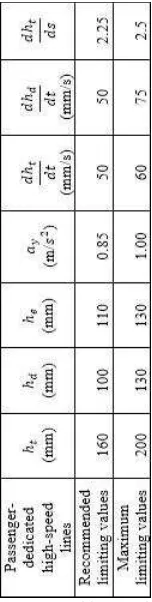
Table 1. Normal and exceptional limit values recommended by TSI and CEN standards (Lindahl, 2001).
TSI: Technical Specification for Interoperability, CEN: European Committee for Standardization.
The explanation of the symbols used in the table is given below:
ℎ = applied cant,
ℎ = cant deficiency,
ℎ = cant excess, = lateral acceleration,
ℎ
= rate of applied cant as a function of time, ℎ� = rate of cant deficiency as a function of time,
ℎ
= rate of applied cant as a function of length.
The cant deficiency (130, 100 mm) and applied cant (200, 160 mm) values recommended for passenger-dedicated high-speed railway lines at 300 km/h speed were obtained by calculating the minimum horizontal curve radii with the following equation (CEN, 2010) and ( TSI, 2000). In the design process, the cant and cant deficiency values were assumed to be 160 mm and 100 mm, respectively.
� � = 11.8 . ����
2
ℎ +ℎ� (1)
Where � = maximum design speed
� � = minimum horizontal curve radius
Table 2 presents the curve radii obtained from Equation (1)
� (km/h) ℎ (mm) ℎ (mm) �mi (m)
300 160 100 4,084
300 160 130 3,662
300 200 100 3,540
300 200 130 3,218
Table 2. Calculated curve radii
To facilitate the application of the resulting values in the field and avoid adverse safety consequences due to mistakes during implementation, the values were rounded up to the nearest multiple of 50, and the minimum horizontal curve radii were assumed to be 3,250 m, 3,550 m, 3,700 m, and 4,100 m. The minimum curve radius was taken as 5,000 m in the design process.
The length of the transition curves was determined by the limiting values of the rate of cant deficiency as a function of time ( ℎ and the rate of cant as a function of length ( ℎ). According to the standards provided by the European Committee for Standardization (CEN), the length of the transition curve should be the longest value derived from the following formulas (CEN, 2010):
� ����
.6 . Δℎ ℎ�
�
− (2)
� Δℎ ℎ −� (3)
Where � = length of transition curve Δℎ = variation of cant deficiency Δℎ= variation of application cant
ℎ� = rate of cant deficiency as a function of time ℎ = rate of application cant as a function of length
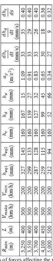
From Equations 2 and 3, the lengths of the transition curves were obtained as 167 m and 71 m, respectively. However, the minimum length of the transition curves was taken as 400 m in the analysis process (Table 3) and 500 m in the design process. Rail transport moving with a constant speed through a curve is subjected to various forces, which affect the safety of the vehicle and the comfort of the traveler. The magnitudes of the forces are the lateral acceleration, rate of lateral acceleration as a function of time, rate of applied cant as a function of time, rate of applied cant as a function of length and rate of cant deficiency as a function of time. Equations 4 to 7 taken from CEN (2010) calculate the forces that arise in horizontal curves for 300 km/h maximum and 200 km/h minimum design speed, constant cant and cant deficiency values and transition curves with 400 m, 450 m and 500 m lengths and horizontal curve radii with of 3,250 m, 3,550 m, 3,700 m, 4,100 m, 5,000 m.
= ����2 � – g .
ℎ
0 (4)
ℎ
= Δℎ . ����
� (5) ℎ� = Δℎ� . ����
� (6) ℎ
= ℎ
�t (7)
Where = lateral acceleration
ℎ = rate of application cant as a function of time g = gravitational acceleration
= track gauge
magnitudes of the forces that arise in curves with 3,250 m, 3,550 m, 3,700 m, 4,100 and 5,000 m radii at 300 km/h maximum and 200 km/h minimum design speed, 160 mm maximum applied cant and 100 mm maximum cant deficiency, respectively.
Table 3. Magnitudes of forces affecting the vehicle in the curves In Table 3, � refers to the transition curve, � � is the minimum design speed, ℎ� represents the equilibrium cant for the maximum design speed, and ℎ � refers to the equilibrium cant for the minimum design speed. The minimum horizontal curve radius was calculated as 4,100 m but it was taken as 5,000 m to provide a comfortable ride and increase the operation speed in future. The parameters assessed for 5,000 m horizontal curve radius and 500 m transition curve do not exceed the limit values given in Table 3. Through these analyses, optimal horizontal geometric parameters were identified to be used in the design process.
2.1.2 Vertical Geometry
Table 4 presents the limit values of vertical curve radius according to the CEN standards.
Passenger-dedicated high-speed lines 250 < V 00 Recommended limiting
values (m)
0.35 . � Minimum limiting values
(m)
0.175 . �
Table 4 Limit values of vertical curve radius (CEN, 2010) The recommended limit values of the vertical curve radius were obtained as 31,500 m for the maximum design speed (300 km/h) but for the implementation, the minimum vertical curve radius value was taken as 30,000 m. During the design process, 0.35 % gradient should be allowed for main tracks. However, the slope of the sliding average profile over 10 km should be less than or equal to 0.25 % or the maximum length of continuous 0.35 % gradient should not exceed 6 km (TSI, 2000). In this study, the maximum gradient was accepted as 2.20 % in the design process.
2.1.3 Selected geometric characteristics
The following geometric parameters were selected to be used in the design of the curves for the improved and alternative passenger-dedicated railway lines:
300 km/h maximum design speed, 200 km/h minimum design speed, 160 mm applied cant,
100 mm cant deficiency,
5000 m minimum horizontal curve radius, 30000 m minimum vertical curve radius, 2.20 % maximum gradient.
Table 5 presents the horizontal geometry design parameters used in the implementations.
�mi (m)
�
(km/h)
� � (km/h)
ℎ
(mm)
ℎ
(mm)
ℎ
(mm)
5000 300 200 160 100 110
Table 5. Limit values for geometric parameters used in the design of the improved and alternative
high-speed railway lines
2.2 Creation of the lines
This section presents the simulation of two railway lines, a geometrically improved existing conventional line and an alternative line for three different land types in accordance with the limit values given in the previous section. After the creation process, the engineering structures and the volume of earthworks required for each line was separately calculated. The determination of these values allows a cost analysis to be performed (Szwaczkiewicz, 2014). Finally, the approximate costs of the lines were calculated and compared.
2.2.1 Implementation 1
The first implementation was carried out on flat-type land, which was not rolling and mountainous. An existing conventional line of 31,837 m length with a minimum curve radius of 850 m, maximum curve radius of 4,000 m, and a maximum gradient of 2.20% was geometrically improved using the design parameters identified in the previous stage.
Figure 1. Routes for the existing and improved conventional lines for Implementation 1
In Figure 1, Line 1 shows the existing conventional railway and its state after improvement, and Line 2 presents an alternative track to the existing conventional line. The lines in blue indicate the straight parts of the tracks while green shows the transition curves and red presents the curves.
The geometrical parameters used for the improvement of the existing line were as follows: Minimum horizontal curve radius 5,000 m, transition curve length 500 m, maximum applied cant 160 mm, minimum vertical curve radius 30,000 m, and maximum gradient 2.20%. For the straight parts of the conventional line, the horizontal curves had a transition curve length of 500 m and a horizontal curve radius of 5,000 m; therefore, the improvement was performed only on the curves. The volume of earthworks and cost calculated for the improvement of 31,818 m long line are given in Tables 6 and 7, respectively.
Cut (m ) Fill (m ) 3,351,632.21 1,053,596.25
Table 6. Volume of earthworks required for the improvement of the existing line on flat land
Cut (TL) Fill (TL) 26,813,057.66 1,126,171.76
Total (TL) 27,939,229.42
Table 7. Approximate total cost of the improvement of the existing line on flat land
In the following stage, a 34,600 m alternative track with 2.20% gradient was created. For this line, the minimum and maximum horizontal curve radii were 5,000 m and 10,000 m, respectively; the minimum and maximum transition curve lengths were 500 m and 1,000 m respectively; the minimum vertical curve radius was 30,000 m; and the minimum and maximum applied cant values were 100 mm and 160 mm, respectively. Tables 8, 9 and 10 present the calculated volume of earthworks, total length of engineering structures and total cost for the alternative line.
Cut (m ) Fill (m ) 6,914,716.96 1,365,259.30
Table 8. Volume of earthworks required for the construction of the alternative line on flat land
Bridge (m) Tunnel (m)
300 0
Table 9. Total length of engineering structures required for the construction of an alternative line on flat land
Cut (TL) Fill (TL) Bridge (TL) 55,317,735.70 12,287,333.70 4,800,000
Total (TL) 72,405,069.38 Table 10. Approximate total cost of constructing an alternative
line on flat land
2.2.2 Implementation 2
The second implementation was carried out on an existing conventional line of 43,000 m in length on rolling-type land. This line had a minimum curve radius of 380 m, maximum curve radius of 3,005 m and maximum gradient of 1.60%.
Figure 2. Routes for the existing and improved conventional line for Implementation 2
In Figure 2, Line 1 in black indicates the existing conventional railway, Line 2 represents the improved state of the conventional railway and Line 3 presents an alternative track to the conventional line. The blue lines represent the straight parts of the tracks, green represents the transition curves, and red indicates the curves.
The following geometrical parameters for the horizontal curves were used to improve the design of the existing line: 5,000 m minimum and 6,000 m maximum horizontal curve radius, 500 m minimum and 600 m maximum transition curve length, 160 mm applied cant, 30,000 m minimum vertical curve is and 2.20%maximum gradient. The volume of earthworks, total length of engineering structures and approximate cost calculated for the improvement of 40,759 m long line are presented in Tables 11, 12 and 13, respectively.
Cut (m ) Fill (m ) 4,197,751.31 1,526,852.01
Table 11. Volume of earthworks required for the improvement of the conventional line on rolling land
Bridge (m) Tunnel (m)
1,870 990
Table 12. Total length of engineering structures required for the improvement of the conventional line on rolling land
Cut (TL) Fill (TL) Bridge (TL)
Tunnel (TL)
33,582,010.51 13,741,668.05 29,920,000 39,600,000 Total (TL) 116,843,678.56 Table 13. Approximate total cost of improving the conventional
line on rolling land
earthworks, total length of engineering structures, and approximate cost calculated for the alternative line.
Cut (m ) Fill (m ) 927,211.80 1,263,432.20
Table 14. Volume of earthworks required for the construction of an alternative line on rolling land
Bridge (m) Tunnel (m) 6,540 1,920
Table 15. Total length of engineering structures required for the construction of an alternative line on rolling land
Cut (TL) Fill (TL) Bridge (TL) Tunnel (TL) 7,417,694.40 11,370,889.79 104,640,000 76,800,000
Total (TL) 200,228,584.20 Table 16. Approximate total cost of constructing an alternative
line on rolling land
2.2.3 Implementation 3
For the third implementation, a mountainous type of land was chosen. The conventional line to be improved was 78,800 m in length with a minimum curve radius of 294 m, maximum curve radius of 3,000 m and a maximum gradient of 2.90%.
Figure 3. Routes for the existing and improved lines for Implementation 3
In Figure 3, Line 1 shows the existing conventional railway, Line 2 represents the improved existing conventional railway line after geometrical improvement, and Line 3 presents an alternative track to the existing conventional line. The straight parts, transition curves and curves are shown blue, green and red, respectively.
To improve the conventional line, the following geometrical parameters were used: horizontal curve radius of 5,000 (min) and 15,000 m (max), transition curve length of 500 m (min) and 1,000 m (max), maximum and minimum applied cant of 70 mm and 160 mm, respectively, minimum vertical curve radius of 30,000 m and maximum gradient of 2.20%. The volume of earthworks, total length of engineering structures and approximate cost calculated for the alternative line of 69,060 m length are given in Tables 17, 18 and 19, respectively.
Cut (m ) Fill (m ) 8,770,928.08 2,779,890.20
Table 17. Volume of earthworks required for the improvement of the conventional line on mountainous land
Bridge (m) Tunnel (m) 1,830 17,330
Table 18. Total length of engineering structures required for the improvement of the conventional line on mountainous land
Cut (TL) Fill (TL) Bridge (TL)
Tunnel (TL)
70,167,424.65 25,019,011.73 29,280,000 693,200,000 Total (TL) 817,666,436.38 Table 19. Approximate total cost of improving the conventional
line on mountainous land
In the second stage of Implementation 3, an 113,170 m alternative track was designed with a 2.20% gradient. For this line, the minimum horizontal curve radius was taken as 5,000 m, maximum horizontal curve radius as 10,000 m, minimum transition curve length as 500 m, maximum transition curve length as 1,000 m, minimum vertical curve radius as 30,000 m, maximum applied cant as 160 mm and minimum applied cant as 100 mm. Tables 20, 21 and 23 present the volume of earthworks, total length of engineering structures and approximate cost calculated for the alternative line.
Cut (m ) Fill (m ) 10,605,170.79 3,742,780.19
Table 20. Volume of earthworks required for the construction of an alternative line on mountainous land
Bridge (m) Tunnel (m) 14,530 29,940
Table 21. Total length of engineering structures required for the construction of an alternative line on mountainous land
Cut (TL) Fill (TL) Bridge (TL) Tunnel (TL) 84,841,366.32 33,685,021.68 232,480,000 1,197,600,000
Total (TL) 1,548,606.39 Table 22. Approximate total cost of constructing an
alternative line on mountainous land
3. RESULTS AND CONCLUSIONS
The two significant findings of the study can be listed as follows: The length of the improved line was shorter than that of the conventional line; however, there was still a need to build new engineering structures and undertake earthworks operations.
For the improved line, the track length and total length of the engineering structures were shorter, the cost of construction was lower and volume of required earthworks was less compared to the alternative line. In addition, it has been observed that in the first implementation, in places where the large-diameter curves designed for high-speed trains overlap the straight sections of the existing conventional line, earthworks need to be undertaken only for curved sections. It is considered that this will help reduce the cost and time.
Although the whole conventional line was not analyzed in this study, from the implementations, it was determined that considering the total length of engineering structures, volume of earthworks and costs, it would be much more feasible and quicker to improve the existing line rather than constructing an alternative line.
ACKNOWLEDGEMENTS
REFERENCES
CEN, 2010. “Railway application-Track alignment design parameters- Track Gauges 1435 and wider-Part 1: Plain line, EN 13803-1:2010”.
Ekim, O., 2007. “Geometrical Specifications and Infrastructure for High-Speed Railways”, Yıldız Technical University, Faculty of Civil Engineering, Department of Transportation, Master's Thesis, Istanbul.
Esveld, C., 2010. “Recent Developments in High Speed Track”, Delft University of Technology, The Netherlands.
Hodas, A., 2014. “Design of Railway Track for Speed and High-speed Railways”, University of Žilina, Fac. of Civil Engineering, Dept. of Railway Engineering, Univerzitná 8215/1, SK-01026 Žilina, Slovak Republic.
Lindahl, M., 2001. “Track Geometry for High-Speed Railways”, Department of Vehicle Engineering Royal Institute of Technology, Stockholm.
Mundrey, J. S., 2010. “Tracking for HighSpeed Trains in India”, RITES Journal, January 2010.
SZWACZKIEWICZ, K., 2014. “Earthwork calculations in various field conditions”, Gdansk University of Technology, Faculty of Railway Transportation and Bridges,
http://www.czasopismologistyka.pl/artykuly-naukowe/send/318-artykuly-na-plycie-cd-3/7113-artykul, Gdansk, Poland (07.09.2016).
TSI, 2000. “European Association for Railway Interoperability (AEIF): Trans-European High-Speed Railway system, Technical Specification for interoperability (TSI), ‘’infrastructure’’ Subsystem, Version A”, April 2000.
Vermeij, D. J., 2000. “Design of a High Speed Track”, Project organisation HSL-Zuid, Utrecth, The Netherlands.