isprsarchives XXXIX B5 489 2012

ERROR DISTRIBUTION EVALUATION OF THE THIRD VANISHING POINT BASED

ON RANDOM STATISTICAL SIMULATION

Chang LI a, * a

College of Urban and Environmental Science, Central China Normal University, Wuhan 430079, China - lichang@mail.ccnu.edu.cn && lcshaka@126.com

Commission V, ICWG V/I

KEY WORDS: Error Distribution, Vanishing Point, Error Ellipse, Random Statistical Simulation, Monte Carlo, RANSAC

ABSTRACT:

POS, integrated by GPS / INS (Inertial Navigation Systems), has allowed rapid and accurate determination of position and attitude of remote sensing equipment for MMS (Mobile Mapping Systems). However, not only does INS have system error, but also it is very expensive. Therefore, in this paper error distributions of vanishing points are studied and tested in order to substitute INS for MMS in some special land-based scene, such as ground façade where usually only two vanishing points can be detected. Thus, the traditional calibration approach based on three orthogonal vanishing points is being challenged. In this article, firstly, the line clusters, which parallel to each others in object space and correspond to the vanishing points, are detected based on RANSAC (Random Sample Consensus) and parallelism geometric constraint. Secondly, condition adjustment with parameters is utilized to estimate nonlinear error equations of two vanishing points (VX, VY). How to set initial weights for the adjustment solution of single image vanishing points is presented. Solving vanishing points and estimating their error distributions base on iteration method with variable weights, co-factor matrix and error ellipse theory. Thirdly, under the condition of known error ellipses of two vanishing points (VX, VY) and on the basis of the triangle geometric relationship of three vanishing points, the error distribution of the third vanishing point (VZ) is calculated and evaluated by random statistical simulation with ignoring camera distortion. Moreover, Monte Carlo methods utilized for random statistical estimation are presented. Finally, experimental results of vanishing points coordinate and their error distributions are shown and analyzed.

* Corresponding author.

1. INTRODUCTION

1.1 Mobile Mapping Systems (MMS)

Mobile Mapping System (MMS) is a new technology emerging in the 1990s for rapid and efficient mapping without ground control (El-Sheimy, 2005), (Graham, 2010). From the 1990s to the beginning of the 21st century, many commercial MMS have been developed, such as GPS VisionTM, GI-EYETM, LD2000TM, ONSIGHTTM, POS/LVTM. Navteq and TeleAtlas also use land-based mobile mapping for navigation database update (El-Sheimy and Schwarz, 1999), (Sullivan D, 2002) and (LI et al., 2009; Scherzinger, 2002).

GPS and Inertial Navigation Systems (INS), have allowed rapid and accurate determination of position and attitude of remote sensing equipment, effectively leading to direct mapping of features of interest without the need for complex post-processing of observed data (Graham, 2010). However, not only does INS have system error, but also it is very expensive. Therefore, in this paper, a low-cost method based on vanishing points is studied and tested in order to substitute INS for MMS in some special land-based scene, such as ground façade where usually only two vanishing points can be detected.

1.2 Vanishing Point

The vanishing point is defined as the convergence point of lines in an image plane that is produced by the projection of the infinite point in real space, which can be used to get three interior parameters (x0, y0, f) and three exterior direction

parameters (φ,ω,κ), (Alantari et al., 2009; Caprile and Torre, 1990; Heuvel, 2003; Lazaros et al., 2007; LI et al., 2011; MAHZAD and FRANCK, 2009; SCHUSTER et al., 1993; XIE and ZHANG, 2004). It is well known that camera parameters can be recovered by the vanishing points of three orthogonal directions. But, three reliable and well-distributed vanishing points are not always available. Even, sometimes only two vanishing points can be gotten (Figure 1). Also, in the scene of ground façade, often only two vanishing points (horizontal orientation VX, plumb line orientation VY) can be detected for façade image, but the vanishing point of depth orientation VZ is difficult to be acquired directly. Thus, the traditional approach based on three vanishing points is being challenged.

Figure 1. Some two vanishing points images (Lazaros et al., 2007)

points (VX,, VY), has important theoretical significance, and also can help to improve the precision of camera calibration. Thus, under the condition of known error ellipses of two vanishing points (VX, VY) and on the basis of the triangle geometric relationship of three vanishing points, the error distribution of third vanishing point (VZ) is discussed and studied.

2. VANISHING POINT MATHEMATICAL MODEL

2.1 Vanishing Point Initial Value Detection

Barnard (Barnard, 1983) introduced the most popular algorithm for the detection of vanishing points based on the construction of the Gaussian sphere. Shufelt (Shufelt, 1999) tries to find vanishing point on the oblique aerial images using Gaussian sphere. Heuvel (Heuvel, 2003) introduced a detection method based on geometric constraints. In 2003, Almansa (Almansa et al., 2003) developed a new method of vanishing point detection without priori information, through using complex probabilistic models. And MAHZAD (MAHZAD and FRANCK, 2009) presented an approach for vanishing point detection based on the theorem of Thales.

In this article, vanishing points are detected to provide initial values for their final adjustment. The steps of detection method are described as follows:

1) Line extraction by Wallis filtering and the LSTM (Least Square Template Matching) algorithm (LI et al., 2009); 2) Angle histogram clustering, that is, linear angle statistics due to aggregation a large number of straight lines in vanishing point direction;

3) RANSAC, which is an iterative method to estimate parameters of a vanishing point approximate coordinate by sampling from a set of observed data containing outliers; 4) Parallelism constraint (Heuvel, 2003), which can be written as the determinant of the mixed product from the normal vectors to the three interpretation planes so as to eliminate straight line dissatisfying the condition of group in vanishing point direction; 5) Calculation the vanishing point coordinates initial value:

( 1)/ 2 coordinate between two straight lines in above support set. 2.2 Adjustment Model

Each straight line grouped into vanishing point direction, e.g., line ij, belonging to this set should pass through the vanishing point V, which can be seen in Figure 2.

Figure 2. Geometric relationships between observational line and vanishing point

Ideally, i, j and V is collinear, so observational equation is:

(

y

V

−

y

i

)(

x

j

−

x

i

) (

−

x

V

−

x

i

)(

y

j

−

y

i

)

=

0

(2) Where: (xi, yi), (xj, yj) and (xv, yv) are the coordinates of i, j and V. Eq.2is linearized by Taylor formula as:

0 coefficient matrix, B is unknown parameter coefficient matrix and W is a closing error vector. The solution of Eq. (5) is: variable weights is as follow (LI and YUAN, 2002):

( 1) ( ) ( ) iteration; variance estimation are:

T T

Where, 2 is the number of necessary observation for Eq. (5). In order to ensure the reliability of adjustment, initial weights should be taken into account. As we know, the angles between straight lines and the lengths of straight line segments affect the accuracy of vanishing point; therefore, prior weight should be determined by these two factors:

Min 2.3 Error Ellipse of Vanishing Point

Caprile (Caprile and Torre, 1990) presented a method to evaluate the accuracy of vanishing point, but arbitrary direction point error can’t be known by this method. Therefore, error ellipse is introduced. According to co-factor matrix propagation law and Eq. (5), the accuracy of vanishing point is estimated by:

2 2

Then, error in point measurement is:

2 2 2 2

0

ˆ

P

ˆ

x

ˆ

y

ˆ

(

xx yy

)

2 2 2

3. VANISHING POINT GEOMETRY AND ITS DISTRIBUTION

3.1 Geometric Relationship among Vanishing Points

According to (ZHANG et al., 2001) , in Figure 3, where S is the

Figure 3. Image geometry with three vanishing points.

3.2 The Solution of the Third Vanishing Point

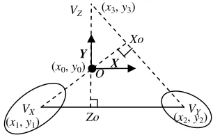
This section, under the condition of known two vanishing points (VX, VY) and the principal point O (x0, y0), how to solve the third vanishing point (VZ) is illustrated as figure 4.

Figure 4. Vanishing points geometry and error ellipse.

VX, VY are the centre of two known error ellipses. And O (x0, y0), which can be set as a coordinate origin, also is the orthocenter of the triangle △VX VY VZ.In figure 4, OZo⊥VXVY, VXOXo⊥ VZVY, thus, VZ is a point of intersection by OZo and VYXo. Let VX(x1, y1), VY(x2, y2) and VZ(x3, y3) be error distributions of three vanishing points. Exactly, (x1, y1) and (x2, y2) are arbitrary points in error ellipses of VX and VY. (x3, y3) is an unknown distribution set about VZ which can be calculated:

3 2 0 1 3 2 0 1

Error ellipse equation can be written:

2_/ 2 2_/ 2 ₁

So, under the right-handed coordinate system XOY (Figure 4):

2 2

3.3 VZ Error Estimation by Random Statistical Simulation

3.3.1 Generating pseudo-random error points

In order to estimate the error distribution of the third vanishing point VZ, firstly, random points of uniform distribution included in error ellipse should be generated. E.g. Figure 5 a) shows a number of random points in error ellipse, which obey uniform distribution (with parameters VX (10, 10), E=10, F=5, φ=π/ 6).

a) Error ellipse filled with points b) Error ellipse filled with circles Figure 5. Generating random points

3.3.2 VZ error distribution pseudo-random simulation On and in the error ellipse VX called set: distribution can be acquired.

3.3.3 VZ error estimation based on Monte Carlo In this section, how to estimate the area size of VZ error distribution is discussed. Suppose the nVsmall circles thrown into an enclosed area by uniform distribution can be aggregated as S_Area, in Figure 5 b). When the N is the larger and the circle is the smaller, S_Area is the much closer to the measure of area. Three algorithms of estimating the area of VZ error distribution are presented as follows respectively.

numbers should be produced? The error ellipse area must be rectangle of error ellipse (in Figure 5). According to geometric probability model that can be called Monte Carlo method here, we have: a total random number can be determined by formula (22). Then, input r and N so that random circles uniformly covering error ellipse VX and VY can be generated. After that, discrete points of VZ error distribution can be gotten by formula (14). Here, we can hypothesis that discrete points VZ are centres of circle with radius r the same as random circles in VX and VY. Thus, area size worth noting that probability is not equivalent to the frequency, so usually

–

best approximation, which can be revised as:

–

ˆ / _V

r= E F n⋅ (24) So the precision of formula (23) can be evaluated by:

– – 2 small circle is? Calculation process is similar to 1). So:

3) In order to avoid error caused by stochastic factor (like above mentioned two methods), we set radius r only as an initial value. After n–_V appears, r is modified by formula

4. EXPERIMENT AND FURTHER WORK

4.1 VZerror estimation based on simulation data

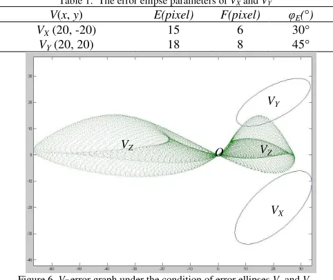
Suppose error ellipse parameters are as below table 1. On the basis of those two error ellipses, the distribution of VZ can be evaluated by formula ( 14). Moreover, its graph is drawn in Figure 6. As we can see, VZ distribution has certain regularity and likes two connected leaves.

Table 1. The error ellipse parameters of VX and VY V(x, y) E(pixel) F(pixel) φE(°)

VX (20, -20) 15 6 30°

VY (20, 20) 18 8 45°

Figure 6. VZ error graph under the condition of error ellipses Vx and Vy

4.2 VZerror estimation based on image data

The input land-based data used in this experiment were shot by a KODAR (PROFESSIONAL DCS Pro SLR/n) non-metric camera with the size of 1000*1500 pixels (compressed), focal length 24mm and the pixel size 0.025mm. Figure 7 b) is the results of line segments extracted and grouped by the directions vanishing points. Furthermore, it is difficult to detect VZ directly.

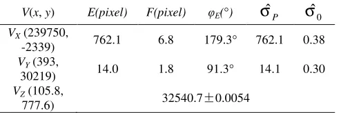
With camera distortion ignored, two error ellipses of VX and VY can be acquired by the adjustment approaches mentioned above,

whose results can be seen in Table 2. σˆ_P is a position error and

0

ˆ

σ

is a standard deviation.

Table 2. The error ellipse parameters of VX and VY for Figure 7 V(x, y) E(pixel) F(pixel) φE(°)

σ

ˆ

_P

σ

ˆ

₀ VX (239750,

-2339) 762.1 6.8 179.3° 762.1 0.38

VY (393,

30219) 14.0 1.8 91.3° 14.1 0.30

VZ (105.8,

777.6) 32540.7±0.0054

The coordinate of the third vanishing point (VZ) is (105.8, 777.6) and its area (32540.7) and error (0.0054) is evaluated by formula (30) and (31) respectively.

4.3 Conclusion and future work

This paper suggests solving vanishing points based on RANSAC and Condition Adjustment with Parameters, which has rigorous theoretical foundation and can greatly eliminate the gross error by RANSAC and iteration method with variable weights. Furthermore, error ellipse, which is calculated by co-factor matrix, is presented to estimate the accuracy of vanishing point. Especially, how to calculate and estimate the third vanishing point (VZ) ant its error distribution is presented based on geometric relationship of vanishing points and random statistical method (Monte-Carlo). A few preliminary theories and methods of evaluation VZ are proposed.

Through the experiment, VZ error graph is drawn by random simulation. Vanishing point (VZ) area and its error is also estimated. The conclusion is that usually the precision of vanishing point is not very high. Moreover, VZ area estimation, in this article, is only simply discussed, so more rigorous solution, such as numerical solution, simulation solution and analytical solution, should be studied deeply in future. This research may expand basic theory, as well as improve or test the universality for the application of vanishing point in order to find a novel and economical way for MMS.

ACKNOWLEDGEMENTS

This work is supported by National Natural Science Foundation of China (NSFC) (Grant No. 41101407), the Natural Science Foundation of Hubei Province, China (Grant No. 2010CDZ005) and self-determined research funds of CCNU from the colleges’ basic research and operation of MOE (Grant No. CCNU10A01001). Heartfelt thanks are also given for the comments and contributions of anonymous reviewers and members of the Editorial team.

References

[1] Alantari, M., Jung, F. and Guedon, J.P., 2009. Automatic and fast method for vanishing point detection. The Photogrammetric Record, 24(127): 246–263. [2] Almansa, A., Desolneux, A. and Vamech, S., 2003.

Vanishing points detection without any a priori information. IEEE Trans. on PAMI, 25(4): 502–507. [3] Barnard, S., 1983. Interpreting perspective images.

Artificial Intelligence, 21.

[4] Caprile, B. and Torre, V., 1990. Using vanishing points for camera calibration. Int. J. Computer Vision, 4(2): 127-140. [5] El-Sheimy, N., 2005. An overview of mobile mapping

systems. FIG Working Week 2005 and GSDI-8—From Pharaos to Geoinformatics, FIG/GSDI,16–21 April, Cairo, pp. 24.

[6] El-Sheimy, N. and Schwarz, K.P., 1999. Navigation Urban

Areas by VISAT-A Mobile Mapping System Integrating GPS/INS/Digital Cameras for GIS Applications. , 45: 275―285.

[7] Graham, L., 2010. Mobile mapping systems overview. Photogrammetric Engineering and Remote Sensing, 76 (3): 222–228.

[8] Heuvel, F.A., 2003. Automation in Architectural Photogrammetry: Line-photogrammetry for the reconstruction from single and multiple images, Delft, Netherlands.

[9] Lazaros, G., George, K. and Petsa, E., 2007. An automatic approach for camera calibration from vanishing points. ISPRS Journal of Photogrammetry and Remote Sensing, 62(1): 64–76.

[10]LI, C., Wu, H., Hu, M. and Zhou, Y., 2009. A Novel Method of Straight-Line Extraction Based on Wallis Filtering for the Close-Range Building, The Asia Pacific Conference on Postgraduate Research in Microelectronics & Electronics. IEEE, Shanghai, China, November 18-20, pp. 290-293.

[11]LI, C., ZHANG, Z. and ZHANG, Y., 2011. Evaluating on the Theoretical Accuracy of Error Distribution of Vanishing Points. Acta Geodaetica et Cartographica Sinica, 43(3): 393-396.

[12]LI, D. and YUAN, X., 2002. Errro processing and reliability theory. Wuhan University Press, Wuhan. [13]LI, D., HU, Q., GUO, S. and CHEN, Z., 2009. Land-based

mobile mapping system with its applications for the Olympic Games. Chinese Science Bulletin, 54(13): 2286-2293.

[14]MAHZAD, K. and FRANCK, J., 2009. precise, automatic and fast method for vanishing point detection. The Photogrammetric Record, 24(127): 246-263.

[15]Scherzinger, B.M., 2002. Inertial aided RTK performance evaluation, In: Proceedings of ION GPS, 24-27

September 2002, Portland, pp. 1429―1433.

[16]School Of Geodesy And Geomatics, W.U., 2003. Error theory and Surveying Adjustment Foundation. Wuhan University Press, Wuhan.

[17]SCHUSTER, R., ANSARI, N. and BANIHASHEMI, A., 1993. Steering a Robot with Vanishing Points. Robotics and Automation IEEE Transactions on Rbotics and Automation, 9(4): 491-498.

[18]Shufelt, J.A., 1999. Performance evaluation and analysis of vanishing point detection. IEEE transactions PAMI, 21(3): 282–288.

[19]Sullivan D, B.A., 2002. Precision kinematic alignment using a Low Cost GPS/INS System, In: Proceedings of ION GPS, 24-27 September 2002, Portland, pp. 1094-1099.

[20]XIE, W. and ZHANG, Z., 2004. Camera Calibration Based on Vanishing Points of Multi-image. ACTA

GEODAETICA et CARTOGRAPHICA SINICA, 33(4): 335-340.