Transport in chemically and mechanically
heterogeneous porous media
V. Two-equation model for solute transport
with adsorption
Azita Ahmadi
a, Michel Quintard
a ,* & Stephen Whitaker
b aL.E.P.T.-ENSAM (UA CNRS), Esplanade des Arts et Me´tiers, 33405 Talence Cedex, France
bDepartment of Chemical Engineering and Material Science, University of California at Davis, Davis, CA 95616, USA
(Received 30 July 1996; accepted 8 September 1997)
In this paper we develop the two-equation model for solute transport and adsorption in a two-region model of a mechanically and chemically heterogeneous porous medium. The closure problem is derived and the coefficients in both the one- and two-equation models are determined on the basis of the Darcy-scale parameters. Numerical experiments are carried out for a stratified system at the aquifer scale, and the results are compared with the one-equation model presented in Part IV and the two-equation model developed in this paper. Good agreement between the two-equation model and the numerical experiments is obtained. In addition, the two-equation model is used, in conjunction with a moment analysis, to derive a one-equation, non-equilibrium model that is valid in the asymptotic regime. Numerical results are used to identify the asymptotic regime for the one-equation, non-equilibrium model. q1998 Elsevier Science Limited.
Key words:porous media, solute transport, adsorption, mathematical modelling.
NOMENCLATURE
agk ¼Agk=Vj, interfacial area per unit volume, m¹
1 . Agk ¼ area of the g–k interface contained in the
averaging volume,Vj, m2
Abj ¼Ajb, area of theb–jinterface contained in the averaging volume,V, m2
Ahq ¼Aqh, area of the boundary between theh and q-regions contained with the large-scale averag-ing volume,V`, m2
bhh vector field that maps=fhchihgh ontoc˜h, m.
bhq vector field that maps=fhcqiqgqontoc˜h, m.
bqq vector field that maps=fhcqiqgqontoc˜q, m.
bqh vector field that maps=hchihghontoc˜q, m.
cg point concentration in theg-phase, mol m¹3.
hchih Darcy-scale intrinsic average concentration for theb–jsystem in theh-region, mol m¹3
.
hcqiq Darcy-scale intrinsic average concentration for theb–jsystem in theq-region, mol m¹3
.
fhchihg h-region superficial average concentration,
mol m¹3 .
fhchihgh ¼J
¹1
h fhchihg,h-region intrinsic average
concen-tration, mol m¹3 .
{hci} ¼ JhfhchihghþJqfhcqiqgq, large-scale intrinsic
average concentration, mol m¹3 . ˜
ch ¼ chih¹ fhchih
h
, spatial deviation concentra-tion for theh-region, mol m¹3.
fhcqiqg q-region superficial average concentration,
mol m¹3.
fhcqiqgq ¼ Jq¹1fhcqiqg, q-region intrinsic average
concentration, mol m¹3. ˜
cq ¼ cqiq¹ fhcqiq
q
, spatial deviation concentra-tion for theq-region, mol m¹3.
Dp
h dispersion tensor for theb–jsystem in the
h-region, m2s¹1 .
Dp
q dispersion tensor for theb–jsystem in the
q-region, m2s¹1 .
Dpp
hh dominant dispersion tensor for theh-region
trans-port equation, m2s¹1 .
Printed in Great Britain. All rights reserved 0309-1708/98/$ - see front matter
PII: S 0 3 0 9 - 1 7 0 8 ( 9 7 ) 0 0 0 3 2 - 8
59
Dpp
hq coupling dispersion tensor for theh-region
trans-port equation, m2s¹1 .
Dpp
qq dominant dispersion tensor for theq-region
trans-port equation, m2s¹1 .
Dpp
qh coupling dispersion tensor for theq-region
trans-port equation, m2s¹1 .
Dpp large-scale, one-equation model dispersion tensor, m2s¹1.
g gravitational acceleration vector, m s¹2.
g magnitude of the gravitational acceleration vector, m s¹2.
I unit tensor
Keq ¼]F=]cg¼]F=]hcgig, adsorption equilibrium
coefficient, m.
K ¼ agkKeq/eg, dimensionless adsorption equilib-rium coefficient for thej-region.
Kh ¼ (ejagk)h=ehÿ]F=]hchih
, dimensionless equilib-rium coefficient for theh-region.
Kq ¼ (ejagk)q=eqÿ]F=]hcqiq
, dimensionless equilib-rium coefficient for theq-region.
,i i¼1,2,3, lattice vectors, m. ,h length scale for theh-region, m. ,q length scale for theq-region, m.
Lc length scale for the region averaged concentra-tions, m.
L aquifer length scale, m.
LH length scale of the aquifer heterogeneities, m. nhq ¼ ¹nqh, unit normal vector directed from the
h-region towards theq-region.
rj radius of the averaging volume, Vj, for the
j-region, m.
ro radius of the averaging volume,V, for theb–j system, m.
hvbih Darcy-scale, superficial average velocity in the h-region, m s¹1.
fhvbihgh intrinsic regional average velocity in theh-region, m s¹1.
hvbiq Darcy-scale, superficial average velocity in the q-region, m s¹1
.
fhvbiqgq intrinsic regional average velocity in theq-region, m s¹1.
superficial average velocity, m s¹1.
Vh volume of theh-region contained in the averaging volume,V`, m
3 .
Vq volume of theq-region contained in the averaging volume,V`, m
3 .
V` large-scale averaging volume for theh–qsystem,
m3.
Greek symbols
a* mass exchange coefficient for the h–q system, s¹1.
Dispersion in heterogeneous media has received a great deal of attention from a variety of scientists who are con-cerned with mass transport in geological formations. It is commonly accepted that dispersion through natural systems such as aquifers and reservoirs involves many different length scales, from the pore scale to the field scale. If one considers the solute transport in such formations, these multiple scales may lead to anomalous and non-Fickian dispersion at the field scale.1–4Here we need to be precise and note that anomalous dispersionrefers to the interpre-tation of field-scale data that does not fit the response of a field-scale homogeneous representation. Similarly, the existence of multiple scales has been related to the observa-tion that dispersivity is field-scale dependent (see a review by Gelhar et al.5), and the theoretical implications of this idea have been discussed extensively.6,7 Clearly, a field-scale description calls for a representation in terms of a heterogeneous domain, and we adopt this point of view in this paper.
1.1 Hierarchical systems
1. the macropore scale, in which averaging takes place over the volume Vj;
2. the Darcy scale, in which averaging takes place over the volume V;
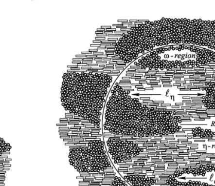
3. the local heterogeneity scale, in which averaging takes place over the volumeV`;
4. the reservoir- or aquifer-scale heterogeneities, which have been identified by the length scaleLHin Fig. 1; no averaging volume has been associated with this length scale since the governing equations will be solved numerically at this scale.
As we suggested in Part IV8, many applications will require the addition of a micropore scale when the k-region illustrated in Fig. 1 contains micropores, and many realistic systems may contain other intermediate length scales either within the b–j system or within the heterogeneities associated with the averaging volumeV`.
When these length scales are disparate, the method of volume averaging can be used to carry information about the physical processes from a smaller length scale to a larger one, and eventually to the scale at which the final analysis is performed. When the length scales are not
disparate, one is confronted with the problem of evolving heterogeneities.4
In this study we assume that the macropore scale, the Darcy scale and the local heterogeneity scale are con-veniently separated. This assumption was also imposed on the analysis presented in Part IV8, and there it led to a Darcy-scale representation of the dispersion process. The analysis required, among other constraints, that
,
k,,gprjp,b,,jprop,h,,q (1)
In the multiple-scale problem under consideration in this paper, Darcy-scale properties are point-dependent, and there is a need for a large-scale description. It is generally assumed9,10 that local heterogeneity-scale permeability variations are ‘stationary’. In other words, gradients of the large-scale averaged quantities, which are characteristic of the regional variations, may be assumed to have negli-gible impact on the change-of-scale problem for character-istic lengths equivalent to the large-scale averaging volume represented by the subscript ` in Fig. 1. Based on this assumption, and provided that the following length-scale constraints are satisfied:
,h,,qpRopLH#L (2)
there is some possibility that a large-scale description exists for the large-scale dispersion process. Here, we mention thepossibleexistence of an averaged description to remind the reader that process-dependent scales are involved in the analysis, and this may lead to conditions that do not permit the development of closed-form volume-averaged transport equations.
Within this framework, we indicated in Part IV8how a local heterogeneity-scale equilibrium dispersion equation
Fig. 1.Averaging volumes in a hierarchical porous medium.
could be derived from the Darcy-scale problem provided that certain length and time scales constraints were fulfilled. In this paper, we remove these latter constraints, and we present an analysis leading to a large-scale, non-equilibrium model for solute dispersion in heterogeneous porous media. The removal of these constraints naturally leads to a better description of the process, and this is clearly demonstrated in our comparison between theory and numerical experiments. The penalty that one pays for this improved description is the increased number of effective coefficients that appear in the two-equation model. If laboratory experiments are required in order to determine these additional coefficients, one is confronted with an extremely difficult task; however, in our theoretical development all the coefficients can be determined on the basis of a single, representative unit cell. This means that all the coef-ficients in the large-scale averaged equations are self-consistent and based on a single model of the local heterogeneities.
The large-scale model that results from our analysis features large-scale properties which are point-dependent with a characteristic length scale, LH, describing the regional heterogeneities. These regional heterogeneities are incorporated into any field-scale numerical description. They will certainly contribute to anomalous, non-Fickian field-scale behaviour, but this behaviour will be taken care of by the field-scale calculations and the large-scale averaged transport equations.
1.2 Large-scale averaging
Within this multiple-scale scheme, we focus our attention on the large-scale averaging volume illustrated in Fig. 2 and thus restrict the analysis to a two-region model of a hetero-geneous porous medium. It is important to understand that the general theory is easily extended to systems containing many distinct regions, and an example of this is given by Ahmadi and Quintard11. Systems of the type illustrated in Fig. 2 are characterized by an intense advection in the more permeable region, while a more diffusive process takes place in the less permeable region. Observations of many similar systems, often referred to as systems with stagnant regions or mobile–immobile regions, have been reported in the literature (see reviews12,13). The expected large-scale behaviour is characterized by large-scale dispersion with retardation caused by the exchange of mass between the different zones. Models proposed for describing solute transport in such cases correspond to the introduction of a retardation factor in the dispersion equation, or a two-equation model for the mobile and immobile regions14–21(see also the reviews cited above12,13). Extensions of these models have been proposed for mobile water in both regions (Skoppet al.22, for the case of small interaction between the two regions, and Gerke and van Genuchten23). In the paper by Gerke and van Genuchten, the solute inter-porosity exchange term is related intuitively to the water inter-porosity exchange
term, i.e. in the case of local mechanical non-equilibrium, and to an estimate of the diffusive part that resembles previously proposed estimates in the case of mobile– immobile systems. It should be noted that the model of Gerke and van Genuchten23 accounts for variably saturated porous media, a case that is beyond the scope of this paper.
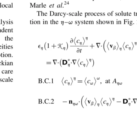
In this paper, we propose a general formulation of these two-equation models using the method of large-scale averaging. We obtain an explicit relationship between the local scale structure and the large-scale equations, suitable for predictions of large-scale properties, which incorporates both coupled dispersive and diffusive contributions. Finally, this methodology is illustrated in the case of dispersion in a stratified system for which we compare the theory both with numerical experiments and with the non-equilibrium, one-equation model of Marle et al.24
The Darcy-scale process of solute transport with adsorp-tion in theh–qsystem shown in Fig. 2 is given by
Here Kh and Kq represent the Darcy-scale equilibrium adsorption coefficients, which may be non-linear functions of the concentrations, hchih and hcqiq. In addition to the solute transport equations, we shall need to make use of the two Darcy-scale continuity equations that take the form
=·vb
h¼0 (7a)
=·vb
q¼0 (7b)
along with the boundary condition for the normal compo-nent of the velocity, which is given by25,26
B:C:3 n
h-region:
q-region:
In our study of the one-equation model presented in Part IV, we made use of the single, large-scale continuity equation; however, in the analysis of mass transport processes using the two-equation model, we shall need the regional forms of the two continuity equations. These can be expressed as:
h-region:
=·fvbhg þ 1 V`
Z
Ahqnhq· vb
hdA¼0 (10a)
q-region:
=·fvbqg þ 1 V`
Z
Aqhnqh· vb
qdA¼0 (10b)
Because the regional velocities are not solenoidal, as are the Darcy-scale velocities contained in eqns (7), one must take special care with the various forms of the regional continuity equations.
In eqns (9), we see various large-scale terms such as ]
ch h h=]
t in eqn (9a) and Jq
vb
q q
cq
q q
in eqn (9b), and we see other terms such as nhqc˜h andvbqc˜q
that involve the spatial deviation quantities. In addition, the inter-region flux is specified entirely in terms of the Darcy-scale variablessuch as vb
hand cq
q
. In the fol-lowing section we shall develop the closure problem which will allow us to determine the diffusive terms such as
˜
Dph·=c˜h and the dispersive terms such as v˜bqc˜q
q
. More importantly, we shall develop a representation for the inter-region flux that is determined entirely by the closure problem. This means that the representation for the inter-region flux is limited by all the simplifications that are made in development of the closure problem.
2 CLOSURE PROBLEM
In the development of a one-equation model, one adds eqns (9a) and (9b) to obtain a single transport equation in which the inter-region flux terms cancel. In that case, the closure problem is used only to determine the effective coefficients associated with diffusion and dispersion. For the two-equation model under consideration here, the closure problem completely determines the functional formof the inter-region flux and the effective coefficients which appear in the representation of that flux. Closure problems can be developed in a relatively general manner; however, the development of a local closure problem requires the use of a spatially periodic model. This means that some very specific simplifications will be imposed on our representation for the inter-region flux and for the large-scale dispersion; however, these simplifications are not imposed on the other terms in eqns (9a) and (9b).
2.1 Inter-region flux
In the development of a two-equation model, we need to represent the inter-region flux terms in a useful form, and this means decomposing that flux into large-scale quantities and spatial deviation quantities. Directing our attention to the h-region transport equation, we make use of the decomposition
ch
h
¼chh h
þc˜h (11)
in order to express the inter-region flux as
1
The second term on the right-hand side of this result is in a convenient form for use with eqn (9a) since the unit cell closure calculations will provide us with values for both
hvbihandDph; however, we need to consider carefully how
we treat the first term. In the derivation of eqn (9a) we made use of the following decomposition for the dispersion
tensor:
Dp
h¼ Dph
h
þD˜ph (13)
When this decomposition is used with eqn (12), we can express the first term on the right-hand side as
1
The large-scale averaged quantities can be removed from the first two terms on the right-hand side of eqn (14); how-ever, we shall leave the gradient of the large-scale average concentration inside the third term to obtain
1
One can show that the first term on the right-hand side of this result is zero for a spatially periodic system. This occurs because the periodicity condition for the velocity,
Periodicity : vb
h(rþ,i)¼ vb
h(r), i¼1,2,3
(16) allows us to write
1
in which Aherepresents the area of entrances and exits for theh-region contained in a unit cell of a spatially periodic porous medium. Use of the divergence theorem and eqn (7) allows us to express eqn (17) as
1
and use of this result with eqn (15) leads to the form
1
result, we make use of the averaging theorem to obtain
¹ 1
V`
Z
AhqnhqdA
· Dp
h
h
·= c
h
h
gh
¼=J
h· Dph
h
·= c
h
h
h
ð20Þ
For a spatially periodic system, =Jh is zero and eqn (20) allows us to express eqn (19) as
1
V`
Z
Ahqnhq· vb
h ch
h
h
¹Dp
h·= ch
h
h
dA
¼ ¹ 1
V`
Z
Ahqnhq·D˜ p
h·= ch
h
h
dA
ð21Þ
We are now ready to return to eqn (12) and express that
inter-region flux according to
1
V`
Z
Ahqnhq· vb
h ch
h
¹Dp
h·= ch
h
dA
¼ 1
V`
Z
Ahqnhq· vb
hc˜h¹Dph·=c˜h¹D˜
p
h·= ch
h
h
dA
ð22Þ
Substitution of this result into eqn (9a) leads to a form of the large-scale average transport equation that is ready to receive results from the closure problem.
h-region:
Here we should note that every term in this result is either a large-scale average quantity or a spatial deviation quantity except for the Darcy-scale velocity, hvbih. This Darcy-scale quantity has not been decomposed like all the other terms, because it will be available to us directly by solution of the Darcy-scale mass and momentum equations for a unit cell in a spatially periodic model of a heterogeneous porous medium. The analogous result for the q-region can be obtained from eqn (9b) and is given by
q-region:
(23a)
In order to evaluate the terms in eqns (23a) and (23b) that contain the spatial deviation concentrations, we need to develop the closure problem forc˜h andc˜q. The
govern-ing differential equation forc˜hcan be obtained by
subtract-ing the intrinsic form of eqn (23a) from the Darcy-scale equation forhchi
h
that is given by eqn (3). We develop the intrinsic form of eqn (23a) by dividing that result by Jh, and this leads to a rather complicated result. However, prior studies27,28clearly indicate that it is an acceptable approx-imation to ignore variations of the volume fraction,Jh,in the development of the closure problem, and this means that the intrinsic form of eqn (23a) can be expressed as
eh 1þKh
Subtraction of this result from eqn (3) leads to
eh 1þKh
Directing our attention to the convective transport term in eqn (25), we make use of the velocity decomposition given by Within the framework of the closure problem, we can use eqns (10) and (18) to obtain
=· v
and since we are ignoring variations of Jh, the continuity equation for the intrinsic regional average velocity takes the form
=· vb h
n oh
¼0 (29)
This result, along with the continuity equation given by eqn (7a) and the decomposition given by eqn (26), can be used to express the convective transport terms in eqn (25) as
Use of the decomposition for the dispersion tensor given by eqn (13) leads to the following representation for the two dispersive fluxes:
When eqns (30) and (31) are used in eqn (25), our transport equation for the spatial deviation concentration takes the form
As a final simplification of this closure problem, we make use of the averaging theorem to write
=c˜
and setting the average of the deviation equal to zero allows us to express this result as
Jh¹1
Multiplication by Dp
h
and this allows us to express eqn (32) in the slightly more compact form given by
If we estimate the accumulation and diffusive terms according to
the closure equation for c˜h will be quasi-steady when the
following constraint is satisfied:
Dphtp
,2hehÿ1þKhq1 (39)
This type of constraint has already been imposed at both the small scale and the Darcy scale, and it is not unreason-able to impose it at the large scale, sinceDp
h will increase
with increasing values of ,h. The convective transport
term and the large-scale dispersive transport term in eqn (36) can be estimated according to
=· vb
and this allows us to neglect the large-scale dispersive transport whenever the length scales of the heterogeneities are constrained by
,h,,qpLc (42)
Moving on to the diffusive terms, we keep eqn (38) in mind and estimate the non-local term as
=· Dp
and we see that this term can also be neglected whenever the constraint given by eqn (42) is satisfied.
On the basis of eqns (39) and (42) we shall simplify the transport equation forc˜hto the following form:
(36)
Here we note that our closure equation will be homogeneous inc˜h if the gradient of the regional average concentration
is zero. For this reason we have identified the two terms involving this gradient as the sources of the c˜h-field. An
analogous form can be derived for the q-region transport equation, and the two will be connected by the interfacial boundary conditions.
On the basis of eqns (4), (5) and (8), we see that the boundary conditions take the form
B:C:1 c
h
h
¼ cq q,
atAhq (45)
B:C:2 n
hq·Dph·= ch
h
¼nhq·Dp
q·= cq q,
atAhq (46)
and when we use the decompositions given by eqn (11), we shall obtain the boundary conditions in terms of the desired spatial deviation concentrations, c˜h and c˜q. This leads us
to the closure problem as follows.
2.2 Closure problem
Periodicity : c˜h(rþ,i)¼c˜h(r), c˜q(rþ,i)¼c˜q(r),
i¼1,2,3 ð47eÞ
Average : c˜h h
¼0, c˜q
q
¼0 ð47fÞ
Here it should be clear that all the sources, or the non-homogeneous terms in this boundary value problem, can be expressed in terms of the two concentration gradients and the concentration difference, i.e.
Sources : = c
h
h
h, =
cq
q
q,
cq
q
q
¹ ch
h
h
ÿ
(47a)
(47b)
(47c)
At this point we have replaced the original problem by a set of large-scale averaged equations and a local-scale closure problem involving the large-scale variables and the spatial deviations. Our objective now is to obtain an approximate solution of this problem. Following ideas developed in the treatment of heat transfer in porous media27,29–32, or in dealing with the flow of a slightly compressible fluid in a heterogeneous porous medium33,34, this suggests representations for the spatial deviation concentrations of the form variables. In terms of these closure variables, there are three closure problems that result from eqns (47), and the first of these is given by
Problem I
Here we have used the vectorschhandcqhto represent the inter-region flux terms according to
chh¼ ¹ 1
and these are related by
chh¼ ¹cqh (50c)
The second closure problem is related to the source, =cqq q
In this case the two constant vectors are defined by
chq¼ ¹ 1
and they are related by
chq¼ ¹cqq (52c)
The third closure problem originates with the exchange source, cq
Here the mass transfer coefficient, a*, is defined by
Rather than work directly with the closure variables,rhand rq, it is convenient to define new variables according to
sh¼rh, sq¼rqþ1 (55)
in order to represent the closure problem for the exchange coefficient in terms of a continuous closure variable. Under these circumstances we express the third closure problem as follows.
In this case the mass transfer coefficient takes the form
ap¼ ¹ 1
These closure problems are similar to those that have been solved previously by Quintard and Whitaker30,35,36, Fabrieet al.37and Quintardet al.32, and they can be used to determine the coefficients that appear in both the two-equation model and the one-two-equation model that was developed in Part IV. The major difference between this development and previously studied two-equation models is associated with the spatial variations of the dispersion tensors due to their dependence on velocity fluctuations. As a consequence, new diffusive source terms appear in the closure problem in the form of the divergence of the deviation of the dispersion tensors. The derivation of the closure problem for the one-equation, equilibrium model is presented in Appendix A.
In order to develop the closed forms of eqn (23a), we substitute the representation forc˜hgiven by eqn (48a) and
make use of the change of variable indicated by eqn (55) to
obtain
Here the various coefficients are defined by
dh¼Jh v˜bhsh¹Dph·=sh
In order to obtain the closed form of theq-region transport equation, we follow the above development from eqn (23b) to arrive at
The coefficients in this case are analogous to those given by eqns (59), and for completeness we list them as
Dpp
In the next section we shall present results for the coeffi-cients given by eqns (59) and (61).
The large-scale equations, eqns (58) and (60), represent a generalized version of two-equation models for describing dispersion and adsorption in such systems, and it is interest-ing to discuss the theoretical status of the linear mass exchange term in these equations. On the basis of the assumptions we have made, the concentration deviations given by eqns (48), coupled with the Darcy-scale problem given by eqns (47), represent a simplified closure scheme for the large-scale averaged equations associated with the h-and q-regions. A general solution would involve a more complicated expression for the exchange between the two effective media, and the retention of the transient form of the closure problem38. In the next section we test the present theory versus numerical experiments obtained for the case of stratified systems.
3 NUMERICAL EXPERIMENTS FOR STRATIFIED SYSTEMS
In this section, we present a complete analysis of the strati-fied system illustrated in Fig. 3 in the absence of adsorption effects. This system has a behaviour typical of the two-region models that have been studied previously24,39–41, while being simple enough to allow for precise analysis. We first obtain Darcy-scale solutions that will serve as numerical experiments for a comparison with theoretical predictions.
3.1 Local problem
The local boundary value problem under investigation is defined below.
Here we note that all the concentrations are now dimen-sionless, so hcaia represents a concentration made dimensionless by some reference concentration, co. The solution of this boundary value problem is trivial in terms of the velocity field, i.e. the velocities are constant in each region. Consequently, the dispersion tensors are constant in each region, and the closure problem can be
simplified in the obvious manner. The two-dimensional con-centration field was obtained by using the numerical model MT3D42.
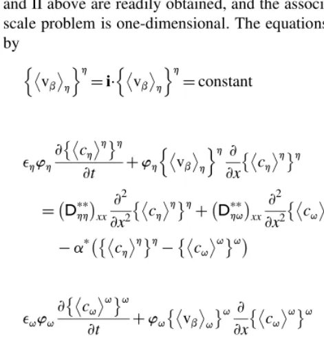
3.2 Closure problems and the large-scale problem
Analytical solutions of the equations of closure problems I and II above are readily obtained, and the associated large-scale problem is one-dimensional. The equations are given by
A complete discussion of associated large-scale boundary conditions is beyond the scope of this study, and we choose the following initial and boundary conditions:
B:C:1 x¼0, chh h¼ cq
In eqns (63), effective properties for the one-dimensional unit cell are given by
Dpp
It is important to note at this point that the periodic system representative of the problem expressed by eqns (62) is constituted of layers twice as large as those represented in Fig. 3, and we have used the appropriate unit cell asso-ciated with this periodic system in deriving eqn (65).
3.3 Numerical methods
Numerical solutions of the large-scale, one-dimensional problem are found by using the following procedure. First, the operator in the transport equation is split into three equations as shown here for theh-region equation:
ehJh
Equations like eqn (66a) are solved by using an explicit second-order scheme43,44, while diffusion equations like eqn (66b) are solved by using a second-order implicit scheme. Finally, eqn (66c) and the similar equation for the q-region are solved analytically for one time-step. The resulting scheme is second-order with negligible numerical dispersion. Several cases were investigated ran-ging from negligible dispersion effects to important disper-sion effects.
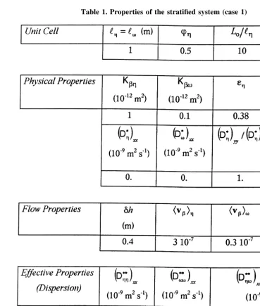
3.3.1 Case 1.
advection, dispersion equation. While these results may seem trivial, they emphasize that with a little additional complexity, i.e. the introduction of a two-equation model, it is possible to take into account mechanisms that would require an extremely complicated one-equation model.
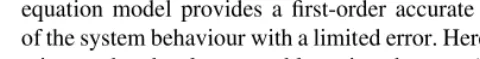
3.3.2 Case 2
The system properties for this case are summarized in Table 2, and the concentration fields obtained fort¼83 10þ6s are plotted in Fig. 6. This figure shows that advection in each strata is the most important mechanism, while some cross-section diffusion is present, and this behaviour clearly
calls for a large-scale, non-equilibrium model. The fields from the numerical experiments, the two-equation model and the one-equation model are plotted in Fig. 7, and there it is seen that the propagation of the front is consider-ably faster in the h-region. Dispersion is negligible; how-ever, mass transfer between the strata is not zero and has a small influence on the concentration field in the region between the fronts. The results indicate relatively good agreement between the numerical experiments and theo-retical calculations, especially for a case that has the reputa-tion for not being ‘Fickian’ in terms of a one-equareputa-tion model. Mass exchange between the strata isunderestimated by the theoretical model, and several explanations can be proposed to explain this phenomenon. We list these as follows:
1. Possible numerical inaccuracies must not be forgot-ten; however, we think that numerical dispersion and
Table 1. Properties of the stratified system (case 1)
accuracy cannot explain all the observed differences. This remark is valid for all cases investigated in this paper, and we shall not repeat this argument in the next set of comments.
2. It has already been observed45that the theory under-estimates the exchanged flux at early times, while it naturally provides better estimates as time increases. This occurs because estimates of the concentration fields provided by the closure problems correspond to a fully established concentration wave in the medium. This is not the case in this particular simula-tion, since there is only a fringe of the strata that is affected by diffusion near the interface.
3.3.3 Case 3
This case corresponds to a system with higher dispersion effects, and the flow properties are given in Table 3. The concentration fields determined at the Darcy scale are plotted in Fig. 8, and all large-scale fields are shown in Fig. 9. The large-scale, one-equation behaviour is still characteristic of non-Fickian behaviour, while the two-equation model provides a first-order accurate description of the system behaviour with a limited error. Here we should reiterate that the closure problem given by eqns (51) through (53) is not exact, and this is generally the case. For especially simple systems, such as Stokes flow in a homo-geneous, rigid porous medium, one can indeed develop exact closure problems46–49; however, the problem under consideration involves transient, convective transport in
heterogeneous porous media and the demands on the closure problem are much greater.
3.3.4 Case 4
The concentration fields at the Darcy scale are shown in Fig. 10 and all large-scale fields in Fig. 11. This case corresponds to much higher dispersion effects. As a result, mass exchange between the strata is increased, and the entire process is closer to large-scale equilibrium. As expected, the difference between numerical experiments and theoretical predictions is small.
Finally, we have performed many numerical experiments under conditions leading to a large-scale equilibrium behaviour by increasing lateral dispersion. Under these circumstances both the two-equation model and the one-equation equilibrium model agree very well with the numerical experiments. This behaviour was of course expected.
4 ASYMPTOTIC BEHAVIOUR
In this section we are interested in the asymptotic behaviour of the stratified system under consideration. In the absence of any adsorption, it has been demonstrated by Marleet al.24 that for sufficiently large times the average concentration obeys rather closely a dispersion equation given by
{e}]fh igc ]t þ vb
]fh igc
]x ¼ D pp
`
ÿ
xx ]2fh igc
]x2 (67)
Fig. 5. Comparison between numerical experiments and 1D large-scale predictions (t¼8310þ6s, case 1).
Fig. 6.Concentration att¼8310þ6
s (case 2).
Fig. 7. Comparison between numerical experiments and 1D large-scale predictions (t¼8310þ6s, case 2).
Fig. 8.Concentration att¼8310þ6
The dispersion coefficient in this equation is given by
Dpp
`
ÿ
xx¼Jh Dph
ÿ
xx
þJq Dpq
ÿ
xxþ
, hþ,q
ÿ 2
12
ehJheqJq
ÿ 2
ehJhþeqJq
ÿ
3 Jh
Dp
h
ÿ
xx
þ Jq
Dp
q
ÿ
xx
" #
vb
b
h¹ vb
b
q
2
ð68Þ
The derivation of this result makes use of the method of moments in a manner similar to the work of Aris50, and these results have been extended to more general, random stratified systems1,51. The estimate of the large-scale asymptotic dispersion coefficient given by eqn (68) was found to agree very well with experimental data24. The one-equation model that was derived in Part IV has exactly the same form as eqn (67), when there is no adsorption, and
this is given by
{e}]{h ic} ]t þ vb
]{h ic}
]x ¼ D pp
ÿ
xx ]2{h ic}
]x2 (69)
This equation is restricted by the approximation
ch
h
h
¼ cq
q
q
¼c ,
large¹scale mass equilibrium ð70Þ
and the predicted dispersion coefficient takes the form
Dpp
ÿ
xx¼Jh Dph
ÿ
xxþJq Dpq
ÿ
xx (71)
This relation is significantly different from the dispersion coefficient represented by eqn (68), which is determined by requiring that the moments of eqn (67) match the moments of the particular process under consideration. While Marle et al.24obtained rather good agreement between theory and
experiment for the case ofpassive dispersionin a stratified system, it would be a mistake to modify eqn (67) with a retardation factor such as ð1þ{K}Þ and expect it to represent accurately an adsorption process.
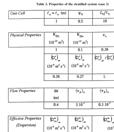
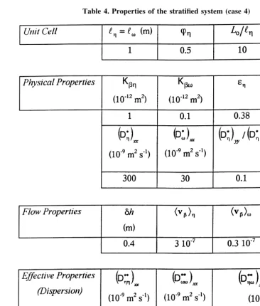
In order to compare our work with eqns (67) and (68), we studied a stratified system, having essentially an infinite length, that was subjected to a step change in the input concentration. Thus we again used eqns (63) through (65) with the lengthLogreat enough for the downstream bound-ary condition to have no effect on the concentration profiles. The physical parameters were taken to be the same as those used in Case 4, so they are given in Table 4 with the exception of Lo/,h, which was of the order of 100. The concentration profiles at a distance of 20 m from the entrance are shown in Fig. 12, from which are seen a variety of different results. The one-equation equilibrium model that is characterized by eqns (69)–(71) clearly
exhibits a lack of dispersion compared with the one-equation non-equilibrium model of Marle et al.24. The results from the two-equation model indicate that the concentration profile for the q-region lies below that for the h-region, and this is required since the velocity in the q-region is a factor of tenless than the velocity in the h-region. At the leading edge of the front, the results from the two-equation model bracket the value predicted by eqns (67) and (68), while at the trailing edge of the front, the non-equilibrium one-equation model of Marle et al.24clearly over-predicts the concentration. The average concentration predicted by the two-equation model is given by
{hci}¼Jh ch
h
h
þJq cq
q
q
(72)
in which ch
h
h
and cq
q
q
are not constrained by eqn (70). We consider this average concentration to be the
best predictor of the large-scale average concentration, and this generally lies below the values predicted by eqns (67) and (68). This means that the time and length-scale con-straints that are imposed on eqns (67) and (68) are not satisfied at a distance of 20 m for the conditions listed in Table 4. The comparison is seen more clearly in Fig. 13, where we present the time derivative of the concentration profiles. These represent values of]{hci}/]t, determined at a distance of 20 m, as a function of time. These curves can also be thought of as concentration profiles for a pulse input condition, and they clearly indicate that eqns (67) and (68) do not predict a symmetric pulse at a distance of 20 m. When the distance is increased to 66.5 m, the agreement between all the models improves significantly, and the results for the concentration profiles are shown in Fig. 14. The one-equation equilibrium model provides the worst representation, while the two-equation model is in good agreement with the work of Marleet al.24. The time deri-vatives of the concentration profiles are shown in Fig. 15, and there we see rather good agreement between the average concentration determined on the basis of the two-equation model and eqn (72) and the one-two-equation non-equilibrium model given by eqns (67) and (68). On the other hand, the one-equation equilibrium model developed in Part IV illustrates rather poor agreement with the other two results.
The direct study of the asymptotic behaviour of the two-equation model is presented in Appendix B, where we show analytically that the asymptotic longitudinal dispersion
coefficient is given by
Dpp
`
ÿ
xx¼ Dpphh
ÿ
xxþ Dpphq
ÿ
xxþ Dppqh
ÿ
xxþ Dppqq
ÿ
xx
þ
eqJq vb
h
n o
¹ehJh vb
q
2
ap e
hJhþeqJq
ÿ ð73Þ
Introducing the expression for a* given by eqn (73), we obtain an expression for the asymptotic longitudinal disper-sion coefficient equal to the one proposed by Marleet al.24. This result suggests the following comments:
1. The two-equation model has an asymptotic behaviour that reflects exactly the behaviour deduced from a direct analysis of the Darcy-scale problem. Since the two-equation model can be applied to more general systems than stratified media, our result represents an important extension of the theory. 2. The value of the asymptotic longitudinal dispersion
coefficient depends ona*. Therefore, the comparison is a test of the validity of the large-scale closure problem. We have presented in Parts I and II a comparison with several estimates of the exchange coefficient published in the literature for purely diffusive problems. They may differ by as much as a factor of 3. The comparison with the result by Marle et al.24shows that the proposed theory gives an exact result.
5 CONCLUSIONS
In this paper we have introduced a first-order version of a two-equation model describing a class of local non-equilibrium dispersion problems in heterogeneous porous media. A comparison with numerical experiments for
Fig. 9. Comparison between numerical experiments and 1D large-scale predictions (t¼8310þ6s, case 3).
Fig. 10.Concentration att¼8310þ6s (case 4).
Fig. 11. Comparison between numerical experiments and 1D large-scale predictions (t¼8310þ6
stratified systems has demonstrated the ability of the two-equation model to describe most of the large-scale non-equilibrium behaviour of such bimodal heterogeneous systems. The agreement was found to be reasonable for a wide range of large-scale Peclet numbers from negligible diffusion/dispersion effects to dominant diffusion/ dispersion effects. In addition to the comparison with numerical experiments, we have also compared our two-equation model with the one-two-equation non-equilibrium model developed by Marleet al.24for the special case of passive dispersion in a stratified system. The asymptotic results are identical, and this represents a successful com-parison with the laboratory experiments that were used by Marleet al.24as a test of their theory. At present there would appear to be no laboratory experiments for the case of dis-persion and adsorption in stratified systems; however, the
numerical experiments can be considered as a reliable veri-fication of the essential features of the two-equation model. An improved model could be achieved with the use of higher-order, transient closure problems. On the other hand, the improvement of the predictions of the two-equation model over those available from the one-equation model is significant, and may be sufficient for many practical purposes. This is a matter of choice for a particular application.
Although interest in two-equation models has long been recognized in the literature, our contribution lies in the introduction of the closure problems that give some reliable link between the lower-scale and the upper-scale structures. The development of numerical methods to solve the closure problems in more general cases could be used in connection with any deterministic or statistical representation of the
heterogeneities, thus providing valuable tools for engineer-ing purposes.
Finally, it must be pointed out that the development presented in this paper is limited to solute transport with negligible density variations and viscosity variations. Gravity-induced gradients may have a significant
influence on the flow pattern41, and it is well known that viscous fingering may develop when viscosity gra-dients are important, thus affecting dramatically the con-centration field. It is not clear at this point whether these effects can be introduced into the analysis in a simple manner.
Fig. 12.Asymptotic behaviour of the different large-scale models: concentration fields (case 4;x¼20 m).
ACKNOWLEDGEMENTS
This work was completed while Stephen Whitaker was a visitor at the Laboratoire Energe´tique et Phe´nome`ne de Transfert in 1994 and 1996. The support of L.E.P.T. and the Socie´te´ de Secours des Amis des Sciences is greatly appreciated. Partial support for Michel Quintard from INSU/PRH is gratefully acknowledged.
APPENDIX A: CLOSURE FOR THE ONE-EQUATION MODEL
In Part IV we expressed the one-equation equilibrium model as
{e} 1ð þ{K}Þ]{h ic}
]t þ=·
ÿ
vb
{h ic}
¼=·ÿDpp·={h ic}
(A1)
Fig. 14.Asymptotic behaviour of the different large-scale models: concentration fields (case 4;x¼66.5 m).
in which the large-scale dispersion tensor is defined by
In order to derive these two results from the two-equation model presented in this paper, we first add eqns (58) and (60) and impose the approximations
c
Use of the definitions
{e} 1ð þ{K}Þ ¼eh 1þKh
allows us to simplify this result to obtain the traditional accumulation and convective transport term according to
{e} 1ð þ{K}Þ]{h ic}
In order to determine the form of the overall dispersion tensor, we recall the definitions of the four dispersion tensors in the above equation, given by
Dpp
These representations need to be arranged in a form that will allow us to extract the relation given by eqn (A2), and we begin this rearrangement with eqn (A8a) to obtain
Dpphh¼Jh Dph· Iþ=bhh
We can remove the regional average from the averaging
process to obtain
and then use the averaging theorem in order to express this term as
Here we have ignored variations ofJh, since we are work-ing with the equations of closure problems I and II above. From eqn (49) we have
bhh
h
¼0 (A12)
and so eqn (A10) takes the form
Dp
Use of this result in eqn (A9) allows us to express Dpp
hh in
which is more conveniently written as
Dpp
If we repeat this procedure with eqns (A8b), (A8c) and (A8d), we obtain
If we sum these four equations, we begin to obtain some-thing that resembles the definition given by eqn (A2):
and the resemblance becomes clearer when we make use of the combined closure variables defined by
bh¼bhhþbhq, bq¼bqhþbqq (A17)
Use of these relations in eqn (A16) leads to
Dpp make use of the two boundary conditions given by eqns (49) and (51) to conclude that
Dpp
Use of this result with eqn (A7) provides the more compact form of the one-equation model given by
{e}ÿ
In order to calculate values of the dispersion tensor,D**, we need the closure problem that produces the closure variables bhandbq. On the basis of the definitions given by eqn (A17) and the following definitions for the constants in the two-equation model closure problems:
ch¼chhþchq, cq¼cqhþcqq (A21)
we can add eqns (49) and (51) to obtain
=· v
At this point we are ready to move on to the non-traditional convective transport terms in eqn (A20), and from eqns (59) and (61) we have
Use of the definitions of the closure variables given by eqn (A17) allows us to add pairs of these equations to obtain
uhhþuhq¼ ¹ 1
On the basis of the boundary condition given by eqn (8):
B:C:3 n
we can add eqns (A24a) and (A24b) to obtain
uhhþuhqþuqhþuqq
Integrating eqn (A22c) over the areaAhqindicates that the two integrals in this result sum to zero:
uhhþuhqþuqhþuqq¼0 (A27)
so eqn (A20) simplifies to
We refer to this form as the one-equation equilibrium model, since it is based on the condition of large-scale equilibrium.
APPENDIX B: MOMENT ANALYSIS OF THE TWO-EQUATION MODEL
A complete analysis of the three-dimensional moments associated with the two-equation model can be found in Zanotti and Carbonell29. In this Appendix, we present a similar analysis with the emphasis on the asymptotic behaviour of the system as a whole, i.e. the average con-centration for the two regions, in order to compare our work with that of Marleet al.24.
We consider a one-dimensional, large-scale flow des-cribed by the two-equation model given by
ehJh
We consider the special case of an infinite medium with the following boundary condition:
along with a similar condition for all derivatives of the concentrations. We adopt the following change of variable:
X¼x¹Vrt={e} (B3)
so that eqns (B1) takes the form
ehJh
We define the spatial moments associated with the
concentration fields as
Multiplying eqns (B4) by Xn and integrating by parts, we obtain the following set of governing equations for the moments:
These equations can be solved sequentially, starting with moments of order zero. All calculations presented below have been performed within SCIENTIFIC WORK-PLACEyusing the MAPLEylibrary.
Moments of order
The set of differential equations to be solved is
ehJh
and the general solution is given by
{e}mh,0¼ehJhgh,0þeqJqgq,0
wheregh,0andgq,0are the initial values. Adding eqns (B8), we obtain the following result:
{e}mo¼ehJhmh,0þeqJqmq,0
In addition, we get
Moments of order 1
From eqns (B6) we get
ehJh
Adding these two equations, we obtain
{e}]m1
The asymptotic behaviour is such that
lim
The reference velocity that makes the right-hand side of this equation equal to zero is
Vr¼ vb
and we shall use this value for Vr in the following paragraphs.
Using symbolic calculus, we were able to obtain the following limits:
Moments of order 2
The governing equations for the moments of order 2 are
ehJh
When these two equations are added, we obtain
{e}]m2
The asymptotic limit is obtained by taking the limit of this equation and using eqns (B15) and (B10) to obtain
{e}]m2
We are now in a position to conclude that the asymptotic behaviour of the two-equation model can be represented by a dispersion equation of the form
{e}]{h ic}
where the asymptotic dispersion coefficient is given by
Dpp
One should note that this development does not make the assumption that the initial conditions are similar for both regions.
REFERENCES
1. Matheron, G. & de Marsily, G., Is transport in porous media always diffusive? A counter example. Water Resour. Res., 1980,16,901–917.
problems in the stochastic convection–dispersion model of solute transport in aquifers and fields soils.Water Resour. Res, 1986,22,77–88.
3. Bacri, J. C., Bouchaud, J. P., Georges, A., Guyon, E., Hulin, J. P., Rakotomalala, N. & Salin, D., Transient non-gaussian tracer dispersion in porous media. In Hydro-dynamics of dispersed media, ed. J. P. Hulin, A. M. Cazabat, E. Guyon & F. Carmona. Elsevier Science (North-Holland), 1990, pp. 249–269.
4. Cushman, J. H. & Ginn, T. R., Nonlocal dispersion in media with continuously evolving scales of heterogeneity. Trans-port in Porous Media, 1993,13,123–138.
5. Gelhar, L. W., Welty, C. & Rehfeldt, K. R., A critical review of data on field-scale dispersion in aquifers.Water Resour. Res., 1992,28(7), 1955–1974.
6. Gelhar, L. W. & Axness, C. L., Three-dimensional stochastic analysis of macrodispersion in aquifers.Water Resour. Res., 1983,19(1), 161–180.
7. Dagan, G., The significance of heterogeneity of evolving scales to transport in porous formation.Water Resour. Res., 1994,30(12), 3327–3336.
8. Quintard, M. & Whitaker, S., Transport in chemically and mechanically heterogeneous porous media IV: Large-scale mass equilibrium for solute transport with adsorption.Adv. Water Resour.,22(1), 33–57.
9. Freeze, R. A., A stochastic–conceptual analysis of one-dimensional groundwater flow in non-uniform homogeneous media.Water Resour. Res., 1975,11,725–741.
10. Dagan, G., Statistical theory of groundwater flow and transport: Pore to laboratory, laboratory to formation, and formation to regional scale.Water Resour. Res., 1986,
22,120–135.
11. Ahmadi, A. & Quintard, M., Large-scale properties for two--phase flow in random porous media.J. Hydrol., 1996,183,
69–99.
12. Brusseau, M. L. & Rao, P. S. C., Modeling solute transport in structured soils: A review.Geoderma, 1990,46,169–192. 13. Gerke, H. H. & van Genuchten, M. T., Evaluation of a
first-order water transfer term for variably-saturated dual-porosity models.Water Resour. Res., 1993,29,1225–1238. 14. Coats, K. H. & Smith, B. D., Dead-end pore volume and
dispersion in porous media.Society of Petroleum Engineers Journal, (1964), 73–84.
15. Gvirtzman, H., Paldor, N., Magaritz, Y. & Bachmat, Y., Mass exchange between mobile freshwater and immobile saline water in the unsaturated zone. Water Resour. Res., 1988,24(10), 1638–1644.
16. Brusseau, M. L., Jessup, R. E. & Rao, P. S. C., Modeling the transport of solutes influenced by multiprocess nonequili-brium.Water Resour. Res., 1989,25(9), 1971–1988. 17. Brusseau, M. L. & Rao, P. S. C., Nonequilibrium and
dis-persion during transport of contaminants in groundwater: Field-scale processes. InContaminant Transport in Ground-water, ed. Kobus & Kinzelbach. Balkema, Rotterdam, 1989. 18. Corre´a, A. C., Pande, K. K., Ramey, H. J. & Brigham, W. E., Computation and interpretation of miscible displacement performance in heterogeneous porous media.SPE Reservoir Engineering, February (1990), 69-78.
19. Peng, C. P., Yanosik, J. L. & Stephenson, R. E., A general-ized compositional model for naturally fractured reservoirs. SPE Reservoir Engineering, 1990,5,221–226.
20. Piquemal, J., On the modelling of miscible displacements in porous media with stagnant fluid. Transport in Porous Media, 1992,8,243–262.
21. Burr, D. T., Sudicky, E. A. & Naff, R. L., Nonreactive and reactive solute transport in three-dimensional heterogeneous porous media: Mean displacement, plume spreading, and uncertainty.Water Resour. Res., 1994,30(3), 791–815.
22. Skopp, J., Gardner, W. R. & Tyler, E. J., Miscible displace-ment in structured soils: Two-region model with small inter-action.Soil Sci. Soc. Am. J., 1981,45,837–842.
23. Gerke, H. H. & van Genuchten, M. T., A dual-porosity model for simulating the preferential movement of water and solutes in structured porous media. Water Resour. Res., 1993, 29,
305–319.
24. Marle, C. M., Simandoux, P., Pacsirszky, J. & Gaulier, C., Etude du de´placement de fluides miscibles en milieu poreux stratifie´.Revue de l’Institut Franc¸ais du Pe´trole, 1967,22,
272–294.
25. Ochoa-Tapia, J. A. & Whitaker, S., Momentum transfer at the boundary between a porous medium and a homogeneous fluid I: Theoretical development.Int. J. Heat Mass Transfer, 1995,38,2635–2646.
26. Ochoa-Tapia, J. A. & Whitaker, S., Momentum transfer at the boundary between a porous medium and a homogeneous fluid II: Comparison with experiment. Int. J. Heat Mass Transfer, 1995,38,2647–2655.
27. Carbonell, R. G. & Whitaker, S., Heat and mass transfer in porous media. InFundamentals of Transport Phenomena in Porous Media, ed. J. Bear & M. Y. Corapcioglu. Martinus Nijhoff, Dordrecht, 1984, pp. 121–198.
28. Whitaker, S., Transport processes with heterogeneous reac-tion. In Concepts and Design of Chemical Reactors, ed. S. Whitaker & A. E. Cassano. Gordon & Breach, New York, 1986, pp. 1–94.
29. Zanotti, F. & Carbonell, R. G., Development of transport equations for multiphase systems I: General development for two-phase systems.Chem. Eng. Sci., 1984,39,263–278. 30. Quintard, M. & Whitaker, S., One and two-equation models for transient diffusion processes in two-phase systems. In Advances in Heat Transfer, Vol. 23. Academic Press, 1993, pp. 369–464.
31. Quintard, M. & Whitaker, S., Local thermal equilibrium for transient heat conduction: theory and comparison with numerical experiments. Int. J. Heat Mass Transfer, 1995,
38,2779–2796.
32. Quintard, M., Kaviany, M. & Whitaker, S., Two-medium treatment of heat transfer in porous media: Numerical results for effective properties.Adv. Water Resour., 1997,20,77–94. 33. Quintard, M. & Whitaker, S., Transport in chemically and mechanically heterogeneous porous media I: Theoretical development of region averaged Equations for slightly com-pressible single-phase flow. Adv. Water Resour., 1996, 19,
29–47.
34. Quintard, M. & Whitaker, S., Transport in chemically and mechanically heterogeneous porous media II: Comparison with numerical experiments for slightly compressible single-phase flow.Adv. Water Resour., 1996,19,49–60. 35. Quintard, M. & Whitaker, S., Convection, dispersion, and
interfacial transport of contaminants: Homogeneous media. Adv. Water Resour., 1994,17,221–239.
36. Quintard, M. & Whitaker, S., Convective and diffusive heat transfer in porous media: 3D calculations of macroscopic transport properties. In EUROTHERM Seminar 96 on Advanced Concepts and Techniques in Thermal Modelling. 1994, pp. I.13–I.19.
37. Fabrie, P., Quintard, M. & Whitaker, S., Calculation of porous media effective properties: computational problems and required unit cell features. In Proceedings of the Con-ference on Mathematical Modelling of Flow Through Porous Media. World Scientific Publishing Co., London, 1995, pp. 166–182.
39. Fattah, Q. N. & Hoopes, J. A., Dispersion in anisotropic homogeneous porous media. J. Hydraul. Eng., 1985, 111,
810–827.
40. Chin, D. A., Macrodispersion in stratified porous media. J. Hydraulic Engineering, 1987,113,1343–1358.
41. Leroy, C., Hulin, J. P. & Lenormand, R., Tracer dispersion in stratified porous media: influence of transverse dispersion and gravity. Journal of Contaminant Hydrology, 1992,11, 51– 68.
42. Zheng, C., MT3D: A modular three-dimensional transport model for simulation of advection, dispersion and chemical reactions of contaminants in groundwater systems. S.S. Papadopulos and Associates, Inc., Bethesda, MD, 1994.
43. Takacs, L., A two-step scheme for the advection equation with minimized dissipation and dispersion errors.Monthly Weather Review, (1985), 113.
44. Bruneau, Ch.-H., Fabrie, P. & Rasetarinera, P., Numerical resolution of in situ biorestoration in porous media, SIAM J. Num. Anal., 1996
45. Grangeot, G., Quintard, M. & Whitaker, S., Heat transfer in packed beds: Interpretation of experiments in terms of
one- and two-equation models. In 10th Int. Heat Transfer Conf., Brighton, vol. 5, 1994, pp. 291–296.
46. Barre`re, J., Gipouloux, O. & Whitaker, S., On the closure problem for Darcy’s law.Transport in Porous Media, 1992,
7,209–222.
47. Quintard, M. & Whitaker, S., Transport in ordered and dis-ordered porous media I: The cellular average and the use of weighting functions.Transport in Porous Media, 1994,14,
163–177.
48. Quintard, M. & Whitaker, S., Transport in ordered and dis-ordered porous media II: Generalized volume averaging. Transport in Porous Media, 1994,14,179–206.
49. Quintard, M. & Whitaker, S., Transport in ordered and dis-ordered porous media III: Closure and comparison between theory and experiment.Transport in Porous Media, 1994,15,
31–49.
50. Aris, R., On the dispersion of a solute in a fluid flowing through a tube. Proc. Roy. Soc. London, A, 1956,
235,67–77.