ORDINAL CLASSIFICATION FOR EFFICIENT PLANT STRESS PREDICTION IN
HYPERSPECTRAL DATA
J. Behmann∗, P. Schmitter, J. Steinr¨ucken, L. Pl¨umer
Institute of Geodesy and Geoinformation, University of Bonn, Meckenheimer Allee 172, Bonn, Germany, [email protected]
Commission VII, WG VII/3
KEY WORDS:Hyper spectral, Classification, Close Range, Agriculture, Feature
ABSTRACT:
Detection of crop stress from hyperspectral images is of high importance for breeding and precision crop protection. However, the continuous monitoring of stress in phenotyping facilities by hyperspectral imagers produces huge amounts of uninterpreted data. In order to derive a stress description from the images, interpreting algorithms with high prediction performance are required. Based on a static model, the local stress state of each pixel has to be predicted. Due to the low computational complexity, linear models are preferable.
In this paper, we focus on drought-induced stress which is represented by discrete stages of ordinal order. We present and compare five methods which are able to derive stress levels from hyperspectral images: One-vs.-one Support Vector Machine (SVM), one-vs.-all SVM, Support Vector Regression (SVR), Support Vector Ordinal Regression (SVORIM) and Linear Ordinal SVM classification. The methods are applied on two data sets - a real world set of drought stress in single barley plants and a simulated data set. It is shown, that Linear Ordinal SVM is a powerful tool for applications which require high prediction performance under limited resources. It is significantly more efficient than the one-vs.-one SVM and even more efficient than the less accurate one-vs.-all SVM. Compared to the very compact SVORIM model, it represents the senescence process much more accurate.
1. INTRODUCTION
Crop stress is induced by environmental factors (e.g. drought, out-of-range temperatures or pathogens) which exceed a critical level (Gaspar et al., 2002, Taiz and Zeiger, 2010). Under pro-longed stress, crop productivity is impaired significantly (Gas-par et al., 2002). In order to meet the demand of agricultural output for an increasing world population (FAO, 2009), agricul-tural science is challenged to enhance crop productivity by im-proving methods of crop management (Davies et al., 2011) and by breeding crops with higher stress tolerance levels (Tester and Langridge, 2010). Breeding and crop management will benefit from phenotyping information: the detection, quantification and visualization of a plant’s stress responses.
In this paper, we focus on drought stress, one of the biggest challenges in global crop production (Pennisi, 2008, Tuberosa and Salvi, 2006). If water shortage exceeds a critical level, a plant initiates stress responses which result in biochemical and morphological adaptations. An important response process, in which resources are reallocated within the plant, is leaf senes-cence. Leaf senescence denotes the final phase of leaf develop-ment and may be induced prematurely under drought stress (Lim and Nam, 2007). It is a spatiotemporal process, which allows the plant to attain the reproductive state under drought conditions. The process is characterized by a degradation of pigments and the relocation of nutrients. It develops continuously and proceeds in patterns from older to younger leaves and, within a leaf, from the tip towards the leaf base (Guiboileau et al., 2010, Lim and Nam, 2007). Furthermore, the senescence process forms an or-dinal order mainly related to pigment degradations (Merzlyak et al., 1999).
In contrast to some plant diseases, drought stress induced senes-cence does not manifest itself in local symptoms. The reallo-cation of resources involves the entire plant - and occurs in all
∗Corresponding author
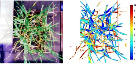
Figure 1: RGB visualization and labeling of a hyperspectral im-age of an barley plant.
plants, even the well watered, to a specific degree. Drought stressed plants are characterized by early and accelerated leaf senescence (Munn´e-Bosch and Alegre, 2004). The aforementioned degra-dation of pigments (particularly chlorophyll) alters the ratio be-tween reflected, absorbed and transmitted radiation (Blackburn, 2007). These changes in spectral characteristics can be observed non-invasively by hyperspectral sensors - even in early stages. The detection and distinction from normal variations requires spec-tral information with high degrees of temporal and spatial resolu-tion.
model selection resulting in adapted and more efficient prediction methods.
In this paper, we present an evaluation of five supervised pre-diction methods for deriving the local stress levels: One-vs.-one Support Vector Machine (SVM), one-vs.-all SVM, Support Vector Regression (SVR), Support Vector Ordinal Regression (SVORIM) and Linear Ordinal SVM classification. In order to compare their accuracy and efficiency, the methods are applied on two data sets - a real world set of drought stress in barley (Hordeum vulgare) and a simulated data set. In the barley data set, the spectra are represented by the values of five Vegetation Indices (VIs).
The rest of this paper is organized as follows: In Section 2 we will describe the data sets used; the aforementioned prediction algo-rithms will be introduced in Section 3. In the fourth section, the results of applying the algorithms on the data sets are presented and discussed. The paper ends in Section 5 with a conclusion.
2. DATA SET
In this study, we compare the performance of different predic-tion algorithms on two data sets. The first data set consists of simulated features and partial overlapping classes with a perfect ordinal order. The second data set consists of VIs derived from hyperspectral images of barley plants under drought stress. The selection of these data sets intends to show the theoretical advan-tages of ordinal classification and how much benefit remains in real world applications.
2.1 Simulated ordinal data
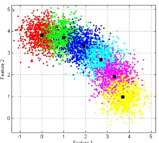
Figure 2: The simulated ordinal data set consists of six Gaussian distributed classes. Each class is represented by a different color, the centroids of the classes are represented by black squares.
The simulated data set consists of six classes and represents a pro-totype of ordinal ordered data. It is used to visualize the discrim-inant functions of the applied prediction algorithms and to show their relevant differences. In order to enable the visualization of the whole feature space, it contains only two features. The ordinal structure is realized by arranging the classes on an arc as shown in Fig. 2. The class centerscihave the same pair-wise distance
of 1 and the samples are Gaussian distributed by∼N(ci,0.2).
The standard deviation of0.2maintains the ordinal order of the classes and, on the other hand, allows distinguishing different re-sult qualities. The data set consists of 5000 labeled instances;
10%are used as training data, the remaining as test data.
Figure 3: Centroids of the cluster for the labeling of the bar-ley data set. The transition from blue to magenta represents the senescence states of the corresponding spectra.
2.2 Hyperspectral features of drought stressed barley plants
The real-world data set is derived from time series of hyperspec-tral images which have been described in detail in (Behmann et al., 2014). In that study, we aimed to detect drought stress in-duced changes in single barley plants as early as possible. Hy-perspectral images were recorded daily for a period of 20 days by a SOC700 hyperspectral imager (Surface Optics, USA). The SOC700 observes the reflectance characteristics from 430 nm to 890 nm in 120 bands; each hyperspectral image has a spatial resolution of 640 x 640 pixels. The images were preprocessed by removing the background using a combination of clustering and setting a threshold as described in (Behmann et al., 2014). Furthermore, the spectral range is reduced due to noise effects at spectral border regions. Examples of hyperspectral images and the spatial variability of the senescence process are shown in Fig. 1 and Fig. 9.
The pixels are labeled by an unsupervised labeling, introduced in (Behmann et al., 2014). The unsupervised labeling uses k-Means to extractkordinal ordered classes whose centroids represent the ordinal order mainly related to chlorophyll degradations of the senescence process. The classes are labeled in ascending order from1tokand the labels are assigned to single pixels.
In this study, the labeling usesk= 10classes and the instances were sampled without spatial context. The final barley data set comprises 211500 test and 21150 training instances, each repre-sented by the values of five Vegetation Indices (VIs). The used VIs were selected by the ReliefF algorithm (Kononenko, 1994) from a basic feature set of 20 VIs (Exelis Visual Information So-lutions, 2012) to reliably exclude irrelevant features and are given in Tab. 1.
Name Formula Reference
ARVI R800−2(R670−R490)
R800+2(R670−R490) (Kaufman and Tanr´e, 1996) RGRI Mean(R500−600)
Mean(R600−700)
(Gamon and Surfus, 1999) RENDVI R750−R705
R750+R705 (Gitelson and Merzlyak, 1994)
SumGreen n1P599i=500Ri (Gamon and Surfus, 1999)
PSRI R680−R500
R750 (Merzlyak et al., 1999)
Figure 4: Decision boundaries of the one-vs.-one SVM classifi-cation model for the simulated data set
3. PREDICTION ALGORITHMS
In machine learning, various supervised algorithms are available for the deduction of models from annotated/labeled training data and the prediction of target variables for unlabeled test data. Clas-sification algorithmspredict discrete classes whereasregression algorithmspredict continuous target values. Ordinal classifica-tionrelies on the assumption of ordinal ordered but discrete classes with a corresponding structure in the feature space.
3.1 Multiclass SVM classifiers
The Support Vector Machine (SVM) (Cortes and Vapnik, 1995) is an established classification method that determines the opti-mal, linear discriminant function between two classes based on the maximum margin principle. Extensions of this method han-dle overlapping classes and even non-linear discriminant func-tions. Multi-class tasks are handled in general by decomposing the multi-class problem in multiple binary class problems (Duan and Keerthi, 2005). The most common decomposing approaches are the one-vs.-one and the one-vs.-all approach.
3.1.1 One-vs.-one SVM The one-vs.-one SVM is the most common multiclass approach. It is based on pairwise classifica-tion, separating all classes from each other (F¨urnkranz, 2002). An example of the decision boundaries for the simulated data set is shown in Fig. 4.
In the learning step, a discrimination function is optimized for each class pair resulting in n∗(n−1)
2 discrimination functions for nclasses. Each optimization uses only the training samples of the regarded pair of classes. The optimization is quite efficient because the amount of training data for a single optimization is small (Duan and Keerthi, 2005). However, the number of opti-mization procedures increases quadratically with the number of classes. A high number of classes result in many, potential un-necessary, discriminate function.
The classification follows themax winsvoting principle in which each discrimination function is applied to the sample (Duan and Keerthi, 2005). Every winning class gets a vote and the class with the highest number of votes is selected as predicted class. This principle is very robust because the contribution of a single, probably misleading discriminant function, is limited. However, for each prediction all of the n∗(n−1)
2 discrimination function
have to be evaluated. For an improved prediction performance, approaches which can reduce the application of discrimination
functions (e.g. directed acyclic graph SVM) were proposed (Platt et al., 1999).
3.1.2 One-vs.-all SVM The one-vs.-all approach consists of discrimination functions which separate one class from all other classes, wherefore it is also called one-vs.-the-rest approach. The discriminant functions are determined by separating the training samples of one class from the aggregated training samples of all other classes. An example of the decision boundaries for the simulated data set is shown in Fig. 5. The model is more com-pact as onlyndiscriminant functions are needed to separate n
classes (Duan and Keerthi, 2005). The classification is based on thewinner takes allprinciple, where the instance is assigned to the class with the maximum probability (Platt, 1999) or, alterna-tively, the highest classification score (normalized distance to the discriminant function). Using posterior probabilities, a stochastic interpretation is enabled and in some applications accuracy im-provements are possible. On the other hand, the determination of the sigmoid functions is computational expensive and addi-tional parameters are required. Therefore, the use of the classi-fication score is preferred in this study focusing the prediction performance.
Figure 5: Decision boundaries of the one-vs.-one SVM classifi-cation model for the simulated data set
The vs.all multiclass approach is less common than the one-vs.-one. It is less robust against outliers because a single mis-leading discriminant function can impair the result quality sig-nificantly (Duan and Keerthi, 2005). However, using well-tuned SVM classifiers comparable result qualities are achievable (Rifkin and Klautau, 2004). Each of the binary discriminant functions suffers from a class imbalance since one class is separated from all the others. Moreover, the usage of all training data for each op-timization can reduce the performance in the training step (Duan and Keerthi, 2005). Whereas in the one-vs.-one approach only two classes contribute to a discriminant function, in the one-vs.-all approach one-vs.-all classes contribute to one-vs.-all discriminant functions. However, the number of SVM evaluations is lower than in the one-vs.-one approach: each of the discriminant functions has to be evaluated for a prediction but the number of functions is lower, especially for higher numbers of classes.
3.2 Support Vector Regression
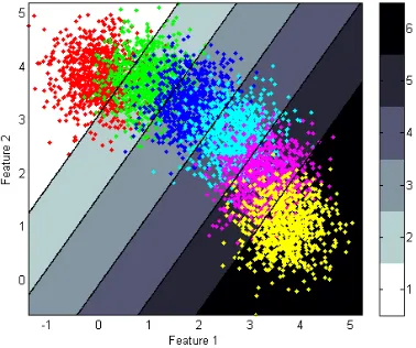
Figure 6: Decision boundaries of the Support Vector Regression model at the simulated data set. The continuous predictions are rounded to an integer to extract the decision boundaries.
basic principle of the binary SVM and results in similar formulas (Vapnik et al., 1997). The formulation is generalizable to non-linear applications by the well-known kernel trick which implic-itly maps the feature vectorsxjto a higher dimensional feature
space and determines their distanceK(xi, xj)in this space.
The regression function is parameterized by the support vectors (SVs)xi, the Lagrangian coefficientsα∗i andαiand the offsetb
The primal optimization function shows the regression approach of the SVR. It is searched for a function that deviates up to a distanceǫfor most of the trainings samples and is as flat as pos-sible (Smola and Sch¨olkopf, 2004). The flatness maximizes the robustness against variations of single features of the input vector
xi. The complexity of the regression model is controlled by the
parameters: toleranceǫ, error weightCand potentially additional kernel parameters.
The SVR was designed to find a regression function based on training instances which are continuously distributed in the fea-ture values as well as the labels (Smola and Sch¨olkopf, 2004). The discrete classes of the ordinal data sets aggregate a high num-ber of instances to a single label value and request a step function. The SVR may approximate the function but its smoothness condi-tion will smooth out the step borders. The SVR is able to model also ordinal data sets but the approximation errors will reduce the prediction quality for ordinal classification data sets. On the other hand, the smooth transition between the classes can be used to represent the uncertainty at the class borders without explicit probability modeling.
The kernels provide linear and non-linear model types. The linear SVR is an extremely compact model but achieves an inferior ac-curacy for both data sets. Therefore, we applied the SVR with a radial basis function (rbf) kernel. This model is able to represent the ordinal transition with a competitive accuracy (Fig. 6). The increased accuracy is accompanied by a higher model complexity due to the non-linear kernel function.
3.3 Ordinal classification
The ordinal classification is applicable in scenarios with discrete labels and known class order (Dembczy´nski et al., 2008). As it
is a special case of the general multi-class scenarios, the intro-duced general prediction methods can be used. Prediction meth-ods which are more adapted to the ordinal structure utilize the additional knowledge about the data set (Behmann et al., 2014) and achieve higher performance measurements. In general, the information about the ordinal data structure is used to reduce the model size by omitting model parts which are not required (Chu and Keerthi, 2007). Different approaches were developed which differ in specific assumptions on data characteristics and the ro-bustness against non-ordinal aspects.
3.3.1 Support Vector Ordinal Regression Support Vector Or-dinal Regression (SVORIM) was developed by (Chu and Keerthi, 2007) in an explicit and an implicit formulation. Both formula-tions determinec−1parallel hyperplanes that separatecclasses and preserves the natural ordinal ordering. The parallelism of the hyperplanes reduces model size and complexity significantly. The linear model comprises only a single weight vectorwfor the whole model and a thresholdbifor each of thec−1 hyper-planes. The optimization is conducted by an adapted sequential minimal optimization (SMO) algorithm, optimizing the ranking of the training instances (Chu and Keerthi, 2007).
Figure 7: Support Vector Ordinal Regression is characterized by parallel discriminant functions resulting in a very compact model.
Fig. 7 shows the position and the orientation of the discriminant functions for the simulated data set. In this context, it becomes apparent that the model is limited regarding non-linear ordinal processes or non-ordinal aspects. However, the SVORIM pre-diction step is extremely efficient and comprises only a multi-plication with the weight vector and the apmulti-plication of thec−1
thresholds. The Support Vector Ordinal Regression represents the most compact model with the lowest model complexity but the low complexity is accompanied by a low adaptability to deviat-ing data characteristics. This may reduce the prediction accuracy on real-world data sets.
3.3.2 Linear Ordinal SVM classification The Linear Ordi-nal classification is defined by discriminant functions between classes which are neighboring on the ordinal scale like at the Sup-port Vector Ordinal Regression (Chu and Keerthi, 2007). Deviat-ing from this approach, the hyperplanes are not forced to be par-allel but are optimized locally (Dembczy´nski et al., 2008). The number of discriminant function remains atc−1but the number of model parameter is significantly higher because each discrimi-nant function has an individual weight vectorwi(Behmann et al.,
2014).
Figure 8: Decision boundaries of the Linear Ordinal SVM clas-sification model for the simulated data set. The overlapping dis-criminant functions are combined by a decision tree for an unam-biguous result.
regions without training instances, the discriminant functions in-tersect each other. Without additional information, these regions of intersections are undefined. Therefore, a tree structure is intro-duced to unambiguously assign a class for each part of the feature space (Behmann et al., 2014). In the tree structure a hierarchy of classes is established by an interval bisection approach. The discriminant functions can be represented by various classifica-tion approaches, e.g. SVM, random forests, logistic regression or naive Bayes.
In this study, we used linear SVMs to enable a reliable compara-bility to the other approaches. In the training step, each discrimi-nant function is optimized on its own with its individual SVM
pa-rameter Ci
(Behmann et al., 2014). The Linear Ordinal SVM classification is represented by the aggregate of all discriminant functions and the tree structure is used for class prediction. In the prediction, the number of evaluation steps is reduced by using the tree structure. Starting from the tree root, the classification is done inlog(c)
steps.
The concept of Linear Ordinal SVM lies between the flexible one-vs.-one multi-class approach and the extreme compact but inflexible Support Vector Ordinal Regression (Chu and Keerthi, 2007). It is able to represent also non-linear ordinal processes but it still relies on the ordinal data characteristics. Non-ordinal aspects cannot be represented due to the reduced number of dis-criminant functions compared to the generic multi-class approaches. The Linear Ordinal SVM classification results in much more com-pact models compared to one-vs.-one classification and may adapt to real-world data sets with only slight losses in accuracy.
4. RESULTS AND DISCUSSION
We evaluate the presented prediction algorithms on two differ-ent data sets. The simulated data set contains ordinal classes in a two-dimensional visualizable feature space. The barley data set contains pixel values with five VIs as features and a ordinal senescence class. This real world data may contain minor non-ordinal aspects and the prediction algorithms have to deal with significant noise effects.
4.1 Simulated ordinal data
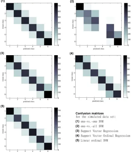
For the simulated data set, the results of the prediction algorithms are very close with the exception of the one-vs.-all SVM (Fig.
Figure 9: Confusion matrix and predicted labels by the Linear Ordinal SVM for a hyperspectral image of a barley plants
10 and Tab. 2). The visualization in Fig. 5 shows that the un-derlying linear model is not able to separate a single class from the remaining classes. As a result, only the classes 1 and 6 are classified correctly, whereas the remaining classes are classified at random. This effect appears always, if a class is not linearly separable from the remaining classes which is in many cases re-lated to a disproportion between the number of features and the number of classes (2 against 6 in the simulated data set). Slight drawbacks are visible at the SVORIM classification which is not flexible enough to follow the arch-shaped ordinal class distribu-tion. The limitation to parallel decision functions requires data with a linear development in each of the features over the whole ordinal structure. The SVR achieves good results for the simu-lated data set due to the flexible rbf kernel. However, the model size increases drastically which impedes the competitiveness to the other prediction methods regarding prediction efficiency (Tab. 2). The one-vs.-one SVM and the Linear Ordinal SVM are
simi-Figure 10: Confusion matrix of the prediction algorithms for the simulated data set with a pure ordinal structure.
Ordi-Method Accuracy [%] MSE # evaluation functions # model parameter
one-vs.-one SVM 78 0.22 15 45
one-vs.-all SVM 54 0.49 6 18
Support Vector Regression (rbf) 76 0.18 1 793
Support Vector Ordinal Regression 74 0.26 5 7
Linear Ordinal SVM 78 0.23 5 15
Table 2: Performance overview on the simulated data set
Method Accuracy [%] MSE # evaluation functions # model parameter
one-vs.-one SVM 83 0.80 45 270
one-vs.-all SVM 46 1.90 10 60
Support Vector Regression (rbf) 66 0.72 1 43986
Support Vector Ordinal Regression 47 1.02 9 14
Linear Ordinal SVM 70 0.82 9 54
Table 3: Performance overview on the barley data set
nal SVM uses a predefined tree structure.
The simulated data set is suitable to compare the different pre-diction algorithms and to highlight specific characteristics. As it shows a pure ordinal process the algorithms are compared under perfect conditions. In contrast, real world data sets contain noise, irrelevant processes and non-ordinal aspects. The performance of the algorithms depends significantly on the robustness against such deviations from perfect conditions.
4.2 Data set: Senescence in barley
The results for the barley data set represents the performance in real world applications (Fig. 11). The differences between the prediction algorithms increase compared to the simulated data set, presumably due to non-ordinal aspects (Tab. 3).
Figure 11: Confusion matrices for the described barley data set.
The prediction algorithms can be separated in two groups: a good accuracy is achieved by the on-vs.-one SVM (83%), the SVR (66%) and the Linear Ordinal SVM (70%); an inferior accuracy is achieved by the on-vs.-all SVM (46%) and the Support Vector Ordinal Regression (47%).
The loss of accuracy of the SVORIM compared to the remain-ing methods is significant and is related to the data characteris-tics. The real-world data incorporating non-linear development of features over the ordinal scale cannot be described by parallel five-dimensional hyperplanes.
Again, the lowest accuracy is achieved by the one-vs.-all SVM. This effect is most probably related to the low number of fea-tures (five feafea-tures and ten classes). Linear discriminant functions seem not to be able to separate one of the ten senescence classes from the others. This effect can be faced by using more features but this would increase data volume as well as model complexity.
The rbf SVR reaches competitive accuracy comparable to the one-vs.-one SVM and the Linear Ordinal SVM. The MSE value is the lowest of all methods related to the continuous predictions. Such output enables further evaluations like probability extrac-tion and a more detailed visualizaextrac-tion. However, its non-linear kernel increases the model size up to an factor of 800. Such a model size prevents a high-throughput prediction as it is required for the efficient evaluation of hyperspectral images. Therefore, it is not suited to be applied for the introduced phenotyping sce-nario.
The one-vs.-one SVM and the Linear Ordinal SVM reach an al-most identical MSE value. However, the accuracy of the one-vs.-one approach is 13% higher. The combination of both result qual-ity measurements reveals the classification characteristics. The one-vs.-one classifies more test samples correctly but if a test sample is misclassified it is more likely assigned to a more distant class. In contrast, the Linear Ordinal SVM assigns the misclas-sified samples in the most cases to one of the two neighboring classes. For the detection of disperse drought stress effects, the overall impression is most important (Fig. 9). It is not or only lit-tle affected by misclassifications to neighboring classes because these classes have nearly the same meaning with regard to the senescence level. Therefore, the higher accuracy of the one-vs.-one SVM approach has only slight positive effects on real-world applications but this advantage is at the expense of a five times higher number of model parameters.
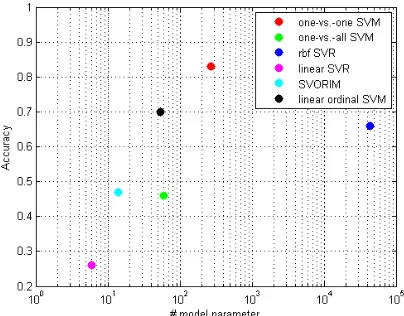
4.3 Prediction efficiency for high-throughput phenotyping
accuracy compared to the Linear Ordinal SVM. Therefore, the user has to choose which characteristic is in the focus. The SVORIM approach is extremely fast but has significant drawbacks in ac-curacy whereas the one-vs.one SVM approach reaches the best accuracy using 20 times more model parameter. The Linear Or-dinal SVM is a compromise between these extrema using a low number of model parameters and reaching an accuracy suitable for many applications (Behmann et al., 2014).
Figure 12: Accuracy related to model size at the example of the barley data set.
5. CONCLUSION
We compared the ordinal classification with established algorithms for classification and regression. The ordinal classification turns out to be a high performant method for the classification of or-dinal data. The one-vs.-one multiclass SVM is the only method with higher accuracy but this is accompanied by a much higher model complexity resulting in 15 times more evaluation steps. The linear regression methods do not reach a comparable accu-racy but they are very compact and fast applied. This example of ordinal data demonstrates that an adaptation of classification algorithms to the specific data characteristics improves the per-formance drastically. Linear Ordinal SVMs have the potential to be applied in upcoming high-throughput phenotyping facilities which will observe a higher number of plants with a larger spatial and temporal resolution. Especially under limited resources like on unmanned aerial vehicles (UAV) or on mobile devices, it will demonstrate the advantages of including knowledge for compact models.
ACKNOWLEDGEMENTS
The authors acknowledge the funding of the CROP.SENSe.net project in the context of Ziel 2-Programms NRW 2007-2013 ”‘Re-gionale Wettbewerbsfhigkeit und Beschftigung (EFRE)”’ by the Ministry for Innovation, Science and Research (MIWF) of the state North Rhine Westphalia (NRW) and European Union Funds for regional development (EFRE) (005-1103-0018) while the preparation of the manuscript. We would like to to thank Christoph R¨omer, Agim Ballvora and Jens L´eon for providing the barley data set.
REFERENCES
Behmann, J., Steinr¨ucken, J. and Pl¨umer, L., 2014. Detection of early plant stress responses in hyperspectral images. ISPRS Journal of Photogrammetry and Remote Sensing 93, pp. 98–111.
Blackburn, G. A., 2007. Hyperspectral remote sensing of plant pigments. Journal of Experimental Botany 58(4), pp. 855–867.
Chu, W. and Keerthi, S., 2007. Support vector ordinal regression. Neural Computation 19(3), pp. 792–815.
Cortes, C. and Vapnik, V., 1995. Support-vector networks. Ma-chine learning 20(3), pp. 273–297.
Davies, W. J., Zhang, J., Yang, J. and Dodd, I. C., 2011. Novel crop science to improve yield and resource use efficiency in water-limited agriculture. The Journal of Agricultural Science 149(Supplement S1), pp. 123–131.
Dembczy´nski, K., Kotłowski, W. and Słowi´nski, R., 2008. Ordi-nal classification with decision rules. In: Mining Complex Data, Springer, pp. 169–181.
Duan, K. and Keerthi, S., 2005. Which is the best multiclass SVM method? an empirical study. In: Proceedings of the 6th International Workshop on Multiple Classifier Systems, Springer, pp. 278–285.
Exelis Visual Information Solutions, 2012. ENVI 5.0 Help. Ex-elis Visual Information Solutions, Colorado.
FAO, 2009. Declaration of the world summit on food security. Food and Agriculture Organisation (FAO) of the United Nations, 16-18 November, Rome. [last access: 12.11.2013].
F¨urnkranz, J., 2002. Round robin classification. The Journal of Machine Learning Research 2, pp. 721–747.
Gamon, J. and Surfus, J., 1999. Assessing leaf pigment con-tent and activity with a reflectometer. New Phytologist 143(1), pp. 105–117.
Gaspar, T., Franck, T., Bisbis, B., Kevers, C., Jouve, L., Haus-man, J. F. and Dommes, J., 2002. Concepts in plant stress physi-ology. application to plant tissue cultures. Plant Growth Regula-tion 37(3), pp. 263–285.
Gitelson, A. and Merzlyak, M., 1994. Spectral reflectance changes associated with autumn senescence of Aesculus hip-pocastanum L. and Acer platanoides L. leaves. Spectral features and relation to chlorophyll estimation. Journal of Plant Physiol-ogy 143(3), pp. 286–292.
Guiboileau, A., Sormani, R., Meyer, C. and Masclaux-Daubresse, C., 2010. Senescence and death of plant organs: Nutrient recy-cling and developmental regulation. Comptes Rendus Biologies 333(4), pp. 382–391.
Kaufman, Y. and Tanr´e, D., 1996. Strategy for direct and indirect methods for correcting the aerosol effect on remote sensing: from AVHRR to EOS-MODIS. Remote Sensing of Environment 55(1), pp. 65–79.
Kononenko, I., 1994. Estimating attributes: analysis and exten-sions of relief. Lecture Notes in Computer Science 784, pp. 171– 182.
Lim, P. O. and Nam, H. G., 2007. Aging and senescence of the leaf organ. Journal of Plant Biology 50(3), pp. 291–300.
Merzlyak, M. N., Gitelson, A. A., Chivkunova, O. B. and Rakitin, V. Y., 1999. Non-destructive optical detection of pigment changes during leaf senescence and fruit ripening. Physiologia plantarum 106(1), pp. 135–141.
Pennisi, E., 2008. The blue revolution, drop by drop, gene by gene. Science 320(5873), pp. 171–173.
Platt, J., 1999. Advances in kernel methods. Vol. 208, MIT Press, chapter Sequential minimal optimization: A fast algorithm for training support vector machines, pp. 98–112.
Platt, J. C., Cristianini, N. and Shawe-Taylor, J., 1999. Large mar-gin dags for multiclass classification. In: nips, Vol. 12, pp. 547– 553.
Rifkin, R. and Klautau, A., 2004. In defense of one-vs-all classi-fication. The Journal of Machine Learning Research 5, pp. 101– 141.
Smola, A. J. and Sch¨olkopf, B., 2004. A tutorial on support vector regression. Statistics and computing 14(3), pp. 199–222.
Taiz, L. and Zeiger, E., 2010. Plant physiology. 5 edn, Sinauer Associates, Sunderland and Mass.
Tester, M. and Langridge, P., 2010. Breeding technologies to in-crease crop production in a changing world. Science 327(5967), pp. 818–822.
Tuberosa, R. and Salvi, S., 2006. Genomics-based approaches to improve drought tolerance of crops. Trends in Plant Science 11(8), pp. 405–412.