FAST DRAWING OF TRAFFIC SIGN USING MOBILE MAPPING SYSTEM
Q. Yaoa, B. Tana, Y. Huanga,∗
a School of Remote Sensing and Information Engineering, Wuhan University,
Wuhan, P.R.China, 430072 - [email protected], tanbin [email protected], [email protected]
ICWG III/VII
KEY WORDS:Traffic Sign,Fast Drawing,Coarse Prediction,Mobile Mapping System (MMS)
ABSTRACT:
Traffic sign provides road users with the specified instruction and information to enhance traffic safety. Automatic detection of traffic sign is important for navigation, autonomous driving, transportation asset management, etc. With the advance of laser and imaging sensors, Mobile Mapping System (MMS) becomes widely used in transportation agencies to map the transportation infrastructure. Although many algorithms of traffic sign detection are developed in the literature, they are still a tradeoff between the detection speed and accuracy, especially for the large-scale mobile mapping of both the rural and urban roads. This paper is motivated to efficiently survey traffic signs while mapping the road network and the roadside landscape. Inspired by the manual delineation of traffic sign, a drawing strategy is proposed to quickly approximate the boundary of traffic sign. Both the shape and color prior of the traffic sign are simultaneously involved during the drawing process. The most common speed-limit sign circle and the statistic color model of traffic sign are studied in this paper. Anchor points of traffic sign edge are located with the local maxima of color and gradient difference. Starting with the anchor points, contour of traffic sign is drawn smartly along the most significant direction of color and intensity consistency. The drawing process is also constrained by the curvature feature of the traffic sign circle. The drawing of linear growth is discarded immediately if it fails to form an arc over some steps. The Kalman filter principle is adopted to predict the temporal context of traffic sign. Based on the estimated point,we can predict and double check the traffic sign in consecutive frames.The event probability of having a traffic sign over the consecutive observations is compared with the null hypothesis of no perceptible traffic sign. The temporally salient traffic sign is then detected statistically and automatically as the rare event of having a traffic sign.The proposed algorithm is tested with a diverse set of images that are taken in Wuhan, China with the MMS of Wuhan University. Experimental results demonstrate that the proposed algorithm can detect traffic signs at the rate of over 80% in around 10 milliseconds. It is promising for the large-scale traffic sign survey and change detection using the mobile mapping system.
1. INTRODUCTION
The detection of traffic signs is an important part of intelligent transportation system. Based on a series of images we get from the Mobile Mapping System (MMS), we focus on finding and identifying the location of potential traffic signs.
Based on the previous EDLine and EDCircle algorithm, a new and fast method is proposed which aims at fitting the circles or ellipses in the images and identifying the possible traffic signs in the images.
Many researchers have made many efforts in recent years to ac-complish the traffic sign detection. An algorithm to detect circle shapes in real images based on Harmony Search algorithm was proposed by Erik Cuevas et al(Cuevas et al., 2012a), who assume that The algorithm uses the encoding of three points as candi-date circles (harmonies) over the edge-only image.Meanwhile, Erik Cuevas also put forward an algorithm based on artificial im-mune systems which aims for multiple circle detection(Cuevas et al., 2012b). The core of their idea is Using a combination of three non-collinear edge points as parameters to determine circles candidates.These two papers advocate the basic principles to find circles in the images. But in the same time, there are also many researches about traffic signs detection. Ming Liang et al(Liang et al., 2013) in Tsinghua University present a model consisting of two modules. The first is for ROI(region of interest) extraction and the second is for recognition. It validates if an ROI belongs to a target category of traffic signs by supervised learning. J.
Stal-∗Corresponding author
2. METHODOLOGY
2.1 Calculate the Color Histogram of Traffic Sign
Traffic signs have certain color combinations and regular shapes. colorsare firstly taken into considerations to extract the regions of interest (ROIs) from an image. In this way we can concentrate on the area where there is a high possibility to have a potential traffic sign rather than going through the whole image. It saves a lot of time. So the main points here are:
1)what color should be chosen and how to choose them to reflect the features of traffic signs in the image without leaving out any one?
2)how to extract the area from the candidate color points?
For the first question: how to choose the proper color, in this re-search w’d like to take color histogram as a solution. Obviously it’s also essential to decide which color space should be taken into consideration. Compared with original RGB color space, HSV has its own advantages. In different conditions such as d-ifferent lighting intensity or complicated background or dd-ifferent photographing angles, it’s much more visual to describe the same color while RGB can’t. Based on the priori knowledge of several colors used int traffic sign, we set up a HSV color index for the standard traffic signs we usually take in the streets.
A={a1, a2....an} (1)
whichArepresents the HSV index of certain kind of standard traffic sign andai stands for the certain color.For each kind of
traffic sign we can set up an index for them. Everyaiis taken
with certain threshold which we will discuss the best threshold in details in later part. Then we count the sum for eachai to
establish the corresponding color histogram.
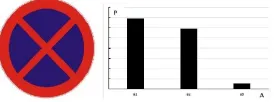
Figure 1: The Histogram of Standard Traffic Sign
The picture above is the color histogram we get for our target.a1
anda2are the main components anda3 can be regraded as the
noise(background)color. The color elementakwith the highest
P(possibility) is regarded as theFeature Color AIand this is the color we will use below.
AI=max(Pi|ai) (2)
According to the feature color we got,we can find all the pixels which are in this color.But they still seem random and irregular. Here comes to the second problem:how to extract the region from the found color points? There is no doubt that these points must have spatial features. Based on clustering, we divided the points into several classes in terms of the distance among the points. In the same way it’s essential to talk about the details. At first we assume the first point as the first class. Then we calculate the distance between the next point and all the central point of exist-ing classes. If the minimum distance exceeds the threshold(after many experiments we find the proper value asd= (W+H)/6, which W,H stands for the width and height of the image) then it belongs to a new class. Otherwise it belongs to the nearest class. After all the points have been classified, we check all the
classes whether it has enough points(consider the scale of im-age we choose 0.1*N as the threshold) and the classes which are large enough can be kept. As long as we found the proper class-es, it’s easy to extract the corresponding ROI from current image knowing the extreme points. Eventually, we find the ROIs and cut down the processing time. From the figure below it’s easy to
Figure 2: The Interest Areas Extracted By Our Algorithm
find that the bottom region is the error ROI we extract in color analysis. Some improvements can be proposed to make it extract precise ROI.Thus, the best threshold will be discussed in the later part.
2.2 Draw the Edge of Traffic Sign
Edge drawing can be divided into four different steps:
1).Firstly, process the image by some filter such as the Gaussian to filter the noise in the image. 2).Secondly, compute the gray scale gradient of each pixel. In this part we can use many mature methods such as Sobel or Prewitt etc. 3).And some pixels which have the local maximum gray gradient in the neighborhood are set as the special points(SP) in the image. And these points mean the pixels have very high probability of being part of an edge. 4).Af-ter we have confirmed all the special points, we get to connect all the SPs dot by dot. From the step 2 we can get the gradient magnitude and its corresponding direction. To be faster, we only choose horizontal or vertical neighborhood for a pixel. Starting from a SP, Edge drawing get its neighbor pixel’s direction and go on(meanwhile record the coordinates of the path). And it will stop when the next dot’s direction is different or the next dot is another SP. So in this procedure we can quickly get the path of the edge.And after all the SPs has been checked, the edge segments of this image could be got.
According to our experiment, after the edge detection, there are many finely edges which severely affected the following proce-dure in the relatively complicated images. So a simple way is chosen to erase these meaningless edges to speed up the process-ing rate. Dependprocess-ing on the length of the edges, we choose to keep or remove them. Longer it is, more information it will take. As-sume that there is a N*N image and an edge whose length is L. If L*L/2≥N*N/100,we think it is a meaningful edge. Otherwise, just abandon it.
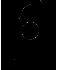
Figure 4: The Result Calculated by EDarwing
2.3 Fit Traffic Sign Shape
After the image de-nosing, the chains of pixels calculated by ED-drawing algorithm(Topal et al., 2010) can be used.With the chains of contiguous pixels, in this part, we mean to split these chain-s to one or more chain-straight line chain-segmentchain-s with EDLine algorith-m(Akinlar and Topal, 2011). According to our first idea, use a certain number of pixels in the sequence and fit a line to these pixels by using the least squares fitting methods. Then compute the distance between this current line and the next pixel. If the distance exceeds a threshold, finish this turn and create a new line segment. If not, add this pixel to the previous ones, fit a new line with the updated pixels to get a more accurate fitting line and loop again (add the next point). The algorithm stops until the distance exceeds a threshold or this chain of pixels has been traversed and processed.
Figure 5 shows the results processed by our algorithm. Figure 6 shows the algorithm used to extract the line segments.
Figure 5: Traffic Sign Processed by EDLine
2.4 Find Circle-arcs and Ellipse-arcs
Differing from the previous definition, in this paper we define a circle arc as a set of a least Two consecutive line segments turning in the same direction. After processing a lot of images, it can be
Figure 6: Algorithm to extract line segments from a pixel chain.
found that many little circle arcs are only divided into 2 line seg-ments. So with this new definition more little circles and details are kept. Here, there are another two main limitations to detect the arcs: the first one is the angle between the two consecutive lines and the second one is the ratio of the two segments length. Given the lines making up the edge segment, calculate the angle between these two consecutive lines and their turning direction by the coordinates. If at least two lines turns in the same direc-tion and the angles among them dont exceed a certain threshold, then calculate the ratio of these two (or more) segments length. If the ratio is close to 1, they may form an arc. Subsequently, by coordinates in the consecutive lines and the least squares fitting methods, fit the arc and add it to the list of arcs. To be more tar-geted and faster, we further divide the arcs into circle-candidate arcs and ellipse-candidate arcs by using FitCircleArcs at first to judge the arcs. If the error doesnt exceed the threshold, add it to the circle-candidate arcs list. If not use FitEllipseArcs to check whether it belongs to ellipse-candidate arcs list. Eventually, split all arcs to these two specific types of arcs. Ultimately, all arcs are classified.
2.5 Find Circles based on clustering
Following the last step, there are two lists of arcs (circle-candidate arcs and ellipse-candidate arcs). It’s obvious that all the circles are combined with the arcs in the lists. And we consider that longer the radius of an arc is, higher the chance of it belonging to a circle (or ellipse) will be. So in this part two assumptions are put forward to shorten the fitting process: Firstly, cluster all the circle-candidate arcs according to the similar center point. Sec-ondly, for every circle cluster, sort the arcs based on descending order of the radius of each arc in the cluster to prepare for the secondary cluster. After these two steps, we can fit all the circles in the image without walking over and computing every arc in every loop which save a lot of time compared with the previous algorithm. For a certain circle-cluster, arcs can be extended un-der several criterions. Given Arc A1 to be extended, the candidate arcs radius should be within 25% of A1’s.
Figure 7: Algorithm to cluster arcs from available line segments.
Figure 8: Arcs detected by our algorithm
fitting up a circle of pixels in the arcs doesnt exceed the thresh-old. This can be regarded as the secondary cluster. Then add A2’s central angle to A1s and substitute A1’s point with A2’s end-point. Here from many observations, we find that if there are more than one arc in the perfect circle, its better to join the arc from a specific direction rather than randomly .So in our algo-rithm we define all arcs’ directions to be anticlockwise. When all the candidate arcs has been found, if A1’s central angle covers at least over 50% of the circumference of its corresponding perfect circle, we make A1 a circle candidate fitted by the least squares fitting methods. If not, the arc is left for ellipse-candidate arcs. And all remaining arcs will be computed by FitEllipseArcs. If within the threshold, they will be added to ellipse-candidate arcs.
2.6 Find Ellipses based on clustering
It’s obvious that all the steps above can only find the nearly per-fect circles. However, in many frames we get, the perper-fect-circle traffic signs will show as ellipses. So we still try to fit ellipse per-fectly. From the ellipse-candidate arcs we get in last step, we can also cluster them into different parts according to similar center
Figure 9: Algorithm to fit circles from every circle cluster
Figure 10: Circle outline detected by our algorithm
point. Then we reorder the arcs based on descending order of the major axis of each arc in every cluster. Given Arc A1 to be extended, the candidate arcs major axis should be within 25% of A1’s. Then check distance between A2s end-point and A1s begin-point and it should not exceed double major axis and the fit error shouldn’t be large. This can be regarded as the secondary cluster. Then A2s central angle is added to A1s and substitute A1s end-point with A2s end-point. Here from many observa-tions, we find that if there are more than one arc in the perfect ellipse, its better to join the arc from a specific direction rather than randomly .So in this part we still define all arcs directions to be anticlockwise. After all the candidate arcs has been obtained, if A1s central angle covers at least over 50% of the circumference of its corresponding perfect ellipse, A1 is regarded as an ellipse candidate fitted by the least squares fitting methods. Here, we use similar methods used in last step to fit ellipse. So we wont show the same parts.
2.7 Fast Traffic Sign Detection and Prediction
frames we got from the MMS, it’s necessary to go through the whole image to extract the interest area. We can record its cor-responding central point and boundary. Subsequently, we only need to detect the edges and fit circle or ellipse in the interest ar-eas.In this way, it sharply decrease the quantity of data needed for edge detection and shorten processing time. And we deem that it’s rational to regard the ellipse or circle fitted in this way as real the traffic signs.Becasue it’s nearly impossible to find a confusion item which is same as traffic sign both in color feature and shape.
However, we still can’t absolutely confirm it. To be more precise we use a statistically coarse prediction as the double-check to reconfirm the existence of traffic sign. The event probability of having a traffic sign over the consecutive frame can be detected statistically.So here the proposed method based on Kalman filter has been taken into consideration.
X(k+ 1|k) =AX′(k|k) +BU(k+ 1)
(3)
whereX(k + 1|k)represents the prediction results in k+1 s-tate(means for the next frame). X′(k|k)stands for the optimal result in k state(means the present frame). U(k+ 1)represents the controlled quantity in k+1 state while A,B are the parameters of the model. And the A,B can be calculated out from the first frame in the video sequence.
P(k+ 1|k) =AP(k|k)AT+Q (4)
whereP(k+ 1|k) represents the corresponding covariance of X(k+1—k) whileP(k|k)stands for the covariance of X(k—k). Q stands for the system covariance. And equation(3)(4) express the prediction for this consecutive system.
X′(k+1|k) =X′(k|k)+K
g(k+1)(Z(k+1)−HX(k+1|k))
(5) hereX′(k+ 1|k)stands for the optimal result in k+1 state and X′(k|k)stands for the optimal result in k state.Z(k+ 1)means the observation value(initial values we use the central points of ellipses in present image.If in the area we can’t fit a ellipse or a circle we use the central points of interest area.In following loops we use the optimal result) whileKg(k+ 1)is the Kalman Gain
which can be calculated as:
Kg(k+ 1) =P(k+ 1|k)HT/(HP(k+ 1|k)HT+R)
(6)
After these, we have gotX′(k+ 1|k), the optimal result in k+1 state(which means the prediction coordinates of corresponding central points in the next frame). Then we have to compute the P(k+ 1|k+ 1)just like below:
P(k+ 1|k+ 1) = (I−Kg(k+ 1)H)P(k|k−1) (7)
In every loop(fromkth frame tok+ 1th frame),we can get a optimal estimated result(predicted central point of the traffic sign in the next frame). Considering the effect of accumulative error, we mean to correct the error in every loop. Started from optimal estimated center,a relatively big area will go through the color analysis and extract a color core.Then based on this color core, we run over color analysis and shape detection in a relative large area. If there is an accepted result in the area, then we regard this frame as a success otherwise it’s a failure. Then if it fails to find a traffic sign, the searching area will be expanded in the next frame and the observation value stays invariable. If it succeed finding one, the area won’t change and the observation value will be replaced as the new central point. Thus in a consecutive frame sequence, we can count the sum of success and failure.
However, there is a problem needed to be discussed. Fristly, as we know, Kalman filter is quite unstable at first because of the
ini-Figure 11: Schematic diagram of correcting error
tial value of A,B parameters in Kalman prediction model are ran-dom.Thus, the error distance will be too large at first. So we try to fix this problem by getting a more precise initial value.Combined with speed datavrecorded by MMS, it’s easy to estimate an ap-proximate coordinate for the following frame and we suppose it as the first Kalman estimation.Then we can go back and get the initial value of A,B. It turns out to be useful in our later tests.
whereP is the optimal estimated central point computed from last frame.Ais the color core got in the first window. Then set A as the center and move the window to A, it will cover more color information and behave much better.
Figure 12: X coordinate of predicted point and measured value
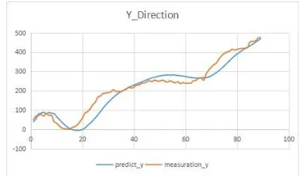
Figure 13: Y coordinate of predicted point and measured value
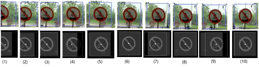
Con=88/90=97.8%.So after this double check is finished and we can confirm the existence of traffic sign. We test our coarse pre-diction in a video and its result turns out to be figure 14.
3. EXPERIMENTAL RESULTS
To measure the performance of our algorithm, a diverse set of images are taken in Wuhan, China with the MMS of Wuhan Uni-versity. It includes traffic signs of different types and colors. And the accuracy and detection speed are presented in this section.
3.1 Color Analysis
At first, the choice of color space is a really problem.Salient fea-tures should be precise and clear enough.The experiments about RGB and HSV color space are shown below: Because of the
Figure 15: Different HSV Threshold Results
different threshold,there are a lot of difference shown from the results.In terms of HSV, we only take H,S(represent the color and its purity)into consideration.Such as 01 and 02,the values of H both are 0to30 330to360,a relative narrow interval for color red.But they differ from S,01 is 0.28 while 02 is 0.5,which means the red found in 02 is purer than 01.So it’s clear that there are lots of error points in 01 while the color points detected in 02 are incomplete.Then we test 03 and 04(exchange the S of 01 and 02,while H is 0 to 60 300 to 360).So we can draw the conclusion that larger the interval is,more error points will be found out.And S should be higher as much as possible,which means the red we find will be more close to real red.
Figure 16: Different RGB Threshold Results
Then it comes to RGB.Because we can’t stimulate the color di-rectly in RGB with the way we analyze the color in our mind. It’s quite blind for us to choose the restrictions. At first, we test 01(R120 G120 B120) and results are quite terrible and mean-ingless.Therefore we add the R value and decrease G,B value step by step such as 02(R125 G115 B115) 03(R135 G105 B105) 04(R145 G95 B95). As the images reflect, less and less points will be found out. In 04 nearly half of the sign has been left out. Therefore we should take a medium value for RGB space and 02 is our best choice. But it’s still hard to judge which space is better. However,in videos, the traffic signs in frames are of-ten affected by different illumination inof-tensity and its color will become quite different.Figure 15 shows the results in low illu-mination while figure 16 in a higher intensity. Figure 01 02 are
Figure 17: Results Obtained By Different Color Space In Normal Light
Figure 18: Results Obtained By Different Color Space In Strong Light
the results got from RGB and 03 04 come from the HSV. Com-pared with its corresponding result in two conditions we can find that while the illumination changes slightly,RGB lost nearly half of right points which means miss a lot of necessary information. Therefore, we assume that RGB is more easy to be affected by illumination change.It’s the RGB’s unstable behavior and poor anti-interference performance that led us to discard it.
And what threshold should be chose to divide the segments?In this part we have tried a lot of experiments.And we pick some salient cases shown in Table 1. whereSumPmeans all the points detected under this threshold whileSumACPstands for the sum of pints belonging to the main class.Classification Accuracy is e-qual toSumACP/SumP which shows the effect of noise.And we precisely got the sum of feature color points is 4435 and the ColorIntegrity calculated asSumACP/4435 illustrates the error classified points ratio.And it should be as close as possi-ble to 100%.After comparing all the cases and we can find case 5 is better.
So it demonstrate that the most proper value of H should be 10-30/300-330 while S is 0.23-0.28.It may differ under different sit-uations.
3.2 Shape Analysis
After color analysis the behaviour of shape detection should also be evaluated.And we use two video sequences as the sample data.
Figure 14: Coarse Prediction Results In a Video
Index Different Cases
1 2 3 4 5 6 7 8
Sum of Points(SumP) 5998 4627 4043 3869 4357 4556 4647 4730
Accurate Classified Points(SumACP) 4750 4377 3887 3869 4357 4556 4647 4730
Classification Accuracy(%) 79.19 94.59 96.14 100 100 100 100 100
Color Integrity(%) 107.10 98.69 87.64 87.24 98.24 102.72 104.78 106.65
H value 60/300 30/330 20/340 10/340 10/330 10/320 10/310 10/300
S value 0.28 0.28 0.28 0.28 0.28 0.28 0.28 0.28
Table 1: Data to find the best threshold in HSV space
Figure 19: Error Ellipse detection result by our algorithm in frame sequence
Figure 20: Error Ellipse detection result by our algorithm in an-other frame sequence
not enough to fit a ellipse. 2.The thickness of the edge affect-s the inner claaffect-saffect-s and the outline claaffect-saffect-s.Thiaffect-s may fit a new ellipaffect-se between two layers or more than two edges.
Figure 21: Several frames in second sequence
3.3 Frame Sequence Analysis
In this part we mean to present its performance in a consecutive frame consequence.And it turns out to be quite precise and fast. In the first sequence it takes nearly 10 milliseconds per frame. Thus, it proves to be fast enough to be real-time algorithm. The traffic sign have been locked and tracked at the beginning. But it performs not that well from a larger angle.Thus, its performance meets our basic expect.
4. CONCLUSIONS AND FUTURE RESEARCH
This paper has introduced a real-time and precise algorithm based on color analysis and shape detection to find the traffic sign in the frame sequence without any restriction on prior experience. We have contributed to the state-of-the-art in two areas:
feature–shape detection to find the ellipse or circle. Therefore its behaviour can be precise and swift.
2)Coarse prediction based on Kalman Filter and double-check s-tatistically.Only simple color and shape conditions are not con-vinced enough to confirm the existence of traffic signs. So we put forward a rough Kalman filter prediction. Through the coarse prediction,we can set up the bond between the current frame and following frame, i.e we can use the center in this frame to predic-t ipredic-ts locapredic-tion in nexpredic-t frame and meanwhile ipredic-t will accelerapredic-te predic-the process. We can count the sum of success and failure frame and compute the confidence coefficient to double check the existence of traffic signs.
We have compared our method with other existing algorithm and observe its performance. A lot of experiments have been taken and its efficiency has been validated.
ACKNOWLEDGEMENTS
The authors are grateful for the support of the program of Low-cost GNSS / INS Deep-coupling System of Surveying and Map-ping (Program NO 2015AA124001), State Key Technology Re-search and Development Program (863), China.
REFERENCES
Akinlar, C. and Topal, C., 2011. Edlines: Real-time line segment detection by edge drawing (ed). In: Image Processing (ICIP), 2011 18th IEEE International Conference on, IEEE, pp. 2837– 2840.
Akinlar, C. and Topal, C., 2013. Edcircles: A real-time circle detector with a false detection control. Pattern Recognition 46(3), pp. 725–740.
Cuevas, E., Ortega-S´anchez, N., Zaldivar, D. and P´erez-Cisneros, M., 2012a. Circle detection by harmony search optimization. Journal of Intelligent & Robotic Systems 66(3), pp. 359–376.
Cuevas, E., Osuna-Enciso, V., Wario, F., Zald´ıvar, D. and P´erez-Cisneros, M., 2012b. Automatic multiple circle detection based on artificial immune systems. Expert Systems with Applications 39(1), pp. 713–722.
Liang, M., Yuan, M., Hu, X., Li, J. and Liu, H., 2013. Traffic sign detection by roi extraction and histogram features-based recogni-tion. In: Neural Networks (IJCNN), The 2013 International Joint Conference on, IEEE, pp. 1–8.
Stallkamp, J., Schlipsing, M., Salmen, J. and Igel, C., 2012. Man vs. computer: Benchmarking machine learning algorithms for traffic sign recognition. Neural networks 32, pp. 323–332.
Topal, C., Akınlar, C. and Genc¸, Y., 2010. Edge drawing: a heuristic approach to robust real-time edge detection. In: Pat-tern Recognition (ICPR), 2010 20th InPat-ternational Conference on, IEEE, pp. 2424–2427.