www.elsevier.com/locate/dsw
An algorithm for the multiparametric 0 –1-integer linear
programming problem relative to the constraint matrix
Alejandro Crema
∗Escuela de Computacion, Facultad de Ciencias, Universidad Central de Venezuela, Apartado 47002, Caracas 1041-A, Venezuela Received 1 January 1998; received in revised form 1 March 2000
Abstract
The multiparametric 0 –1-Integer Linear Programming (0 –1-ILP) problem relative to the constraint matrix is a family of 0 –1-ILP problems in which the problems are related by having identical objective and right-hand-side vectors. In this paper we present an algorithm to perform a complete multiparametric analysis. c2000 Elsevier Science B.V. All rights reserved.
Keywords:Integer programming; Parametric programming; Knapsack problem
1. Introduction
The need for parametric analysis in Mathematical Programming arises from the uncertainty in the data. The most important surveys of parametric methods in integer linear programming (ILP) have been published by Georion and Nauss [4], Holm and Klein [5] and Jenkins [8]. Most work has been done on changes in the right-hand side or in the objective vector with a scalar parameter guiding the perturbation of the data. Changes in elements of the constraint matrix have been considered by Jenkins [7] with a scalar parameter guiding the perturbation in such a manner that for the maximization case the feasible region increases con-tinuously . The multiparametric ILP problem relative to the right-hand-side vector has been considered by Crema [2] and some of the ideas presented here may
∗Fax: 58-2-605-1131 or 58-2-605-2136.
E-mail address:[email protected] (A. Crema).
be considered as generalizations of those presented in that work. In the case of multiple changes on the con-straint matrix, in such a manner that there is no scalar guiding the perturbation, no deep results are known up to now [8,1].
Let L and U be matrices such that L∈Zm×n
andU∈Zm×n withL
ij6Uij for all (i; j)∈I×J =
{1; : : : ; m} × {1; : : : ; n}. Let H = {A:A∈Zm×n;
Lij6Aij6Uij ∀(i; j)∈I ×J}. Let ={(i; j)∈I ×
J:Lij¡ Uij}. In this paper6=∅. LetS⊆H dened
by linear constraints inAijwhere (i; j)∈I×J.
The multiparametric 0 –1-ILP problem relative toS
is a family of 0 –1-ILP problems in which the prob-lems are related by having identical objective and right-hand-side vectors. A member of the family is dened as
(P(A)) max ctx s:t: Ax6b; x∈ {0;1}n
wherec∈Rn; b∈ZmandA∈S.
Because all the constraints can be put in the form
6and for the sake of standardization the members of the family were written in a maximization form with all the constraints in the form6.
We use the following standard notation: ifT is an optimization problem thenF(T) denotes its set of fea-sible solutions, ifDis a matrixDi∗denotes itsith row
vector.
Constraints in the form ¿ can be treated as fol-lows: let us consider the constraint atx¿a0 where
L′
j6aj6Uj′, then we useAi1∗x6bi1=−a0with−U
′
j=
Li1j6Ai1j6Ui1j=−L
′
j.
Equality constraints can be treated as follows: let us consider the constraintatx=a
0whereL′j6aj6Uj′.
In this case we use two constraints,
Ai1∗x6bi1=a0
where
L′
j=Li1j6Ai1j6Ui1j=U
′
j
and
atx¿a0 whereL′j6aj6Uj′
and now the second constraint can be put in the form
Ai2∗x6bi2=−a0such as we explain above. Note that in this case the parameters of constraintsi1andi2 are
not independent and their relations (Ai2j=−Ai1j for allj) must be included to deneS.
We say that a multiparametric analysis is complete after nding an optimal solution forP(A) (if it exists) for all A∈S. In this paper we present an algorithm to perform a complete multiparametric analysis. Our algorithm works by choosing an appropiate nite se-quence of non-parametric ILP problems in such a man-ner that the solutions of the problems in the sequence provide us with a complete multiparametric solution. This kind of approach was introduced by Jenkins [6 –8] to the single parametric case.
In Section 2 we present the theoretical results and the algorithm. Computational experience is presented in Section 3.
2. Theoretical results and the algorithm
LetQ(1) be a non-linear integer problem in (x; A)
dened as
(Q(1)) maxctxs:t: Ax6b; x∈ {0;1}n; A∈S:
Observe thatAij is a decision variable in Q(1) for
all (i; j)6∈.
Remark 1. (i) By construction ofQ(1), ifF(Q(1)) =∅
thenF(P(A)) =∅for allA∈S. (ii) SinceF(Q(1)) is a
nite set, ifF(Q(1))6=∅then there exists an optimal
solution forQ(1).
Lemma 1. Let us suppose that F(Q(1)) 6= ∅ and
let (x(1); A(1)) be an optimal solution for Q(1). Let
W(1)={A:A∈S; Ax(1)6b}.IfA∈W(1) thenx(1) is
an optimal solution forP(A).
Proof. IfA∈W(1)thenx(1)∈F(P(A)). If x∈F(P(A)) then ( x; A)∈F(Q(1)) andctx6ctx(1).
In order to use Remark 1 and Lemma 1 we solve an ILP problem equivalent toQ(1). LetQL(1) be an ILP problem in (x; B) dened as
(QL(1)) max ctx s:t:;
Ui∗x−
X
j∈J
Bij6bi ∀i∈I;
Bij−(Uij−Lij)xj60 ∀(i; j)∈I×J;
x∈ {0;1}n; B∈Zm×n; B
ij¿0 ∀(i; j)∈I×J;
U−B∈S:
Remark 2. Observe that if (i; j)6∈thenUij=Lijand
Bij= 0 and therefore if (i; j)6∈we can delete the
variableBijand the constraintBij−(Uij−Lij)xj60
in order to solveQL(1).
Lemma 2. Let us suppose that(x(1); B(1))∈F(QL(1))
and letA(1)ij =Uij−Bij(1) for all (i; j)∈I ×J.Then;
(x(1); A(1))∈F(Q(1)).
Proof. Since (x(1); B(1))∈F(QL(1)) and from the def-inition ofA(1) we have that
A(1)i∗x
(1)= (U
i∗−B
(1) i∗)x
(1)
=Ui∗x(1)−
X
j∈J
B(1)ij 6bi ∀i∈I:
Lemma 3. Let us suppose that(x(1); A(1))∈F(Q(1))
and let B(1)ij = (Uij−A(1)ij )x (1)
j for all (i; j)∈I ×J.
Proof. SinceA(1)∈S and from the denition ofB(1)
we have that
B(1)ij = (Uij−A(1)ij )x (1) j
6(Uij−Lij)xj(1) ∀(i; j)∈I×J:
Since (x(1); A(1))∈F(Q(1)) and from the denition
ofB(1) we have that
Ui∗x(1)−
X
j∈J
B(1)ij =Ui∗x(1)−(Ui∗−A
(1) i∗)x
(1)
=A(1)i∗x
(1)6b
i ∀i∈I:
Thus, (x(1); B(1))∈F(QL(1)).
Corollary 1. (i)F(Q(1))=∅if and only ifF(QL(1))=
∅. (ii) Let us suppose that F(QL(1)) 6= ∅; let
(x(1); B(1)) be an optimal solution for QL(1); let
A(1)ij = Uij − Bij(1) for all (i; j)∈I × J and let
W(1)={A:A∈S; Ax(1)6b}. Then (ii:1) (x(1); A(1))
is an optimal solution forQ(1);(ii:2)ifA∈W(1)then
x(1) is an optimal solution forP(A).
Remark 3. (i) IfF(QL(1)) =∅thenF(P(A)) =∅for
allA∈Sand the multiparametric analysis is complete. (ii) If S=W(1) then the multiparametric analysis is
complete.
In order to decide whetherS=W(1)we will present
an integer feasibility problem later in this section. In general, suppose thatx(1); : : : ; x(r) andW(1); : : : ;
W(r) are given (r¿1) such that
(i) W(k)={A∈S:Ax(k)6b} 6=∅(k∈ {1; : : : ; r}). (ii) If A∈W(1) thenx(1) is an optimal solution for
P(A).
(iii) IfA∈W(k)−(W(1)∪ · · · ∪W(k−1)) thenx(k) is
an optimal solution forP(A) (k∈ {2; : : : ; r}).
LetQ(r+1)be a non-linear integer problem in (x; A)
dened as:
(Q(r+1)) maxctxs:t: Ax6b; x∈ {0;1}n;
A∈S−(W(1)∪ · · · ∪W(r))
Remark 4. (i) By construction of Q(r+1), if
F(Q(r+1)) =∅then eitherS= (W(1)∪ · · · ∪W(r)) or
F(P(A)) =∅for allA∈S−(W(1)∪ · · · ∪W(r)). (ii)
SinceF(Q(r+1)) is a nite set, ifF(Q(r+1))6=∅then
there exists an optimal solution forQ(r+1).
Lemma 4. Let us suppose that F(Q(r+1)) 6= ∅ and
let(x(r+1); A(r+1)) be an optimal solution forQ(r+1).
LetW(r+1)={A: A∈S; Ax(r+1)6b}.IfA∈W(r+1)−
(W(1)∪ · · · ∪W(r))thenx(r+1)is an optimal solution
forP(A).
Proof. IfA∈W(r+1)−(W(1)∪· · ·∪W(r)) thenx(r+1)∈
F(P(A)). If x∈F(P(A)) then ( x; A)∈F(Q(r+1)) and
ctx6ctx(r+1).
In order to use Remark 4 and Lemma 4 we solve an ILP problem equivalent toQ(r+1). LetMi(k)= (Ui∗−
Li∗)x(k) for all k∈ {1; : : : ; r} and for all i∈I. Let
QL(r+1)be an ILP problem in (x; B; y(1); : : : ; y(r))
de-ned as
(QL(r+1)) max ctx s:t:
(x; B)∈F(QL(1));
Bi∗x(k)+y
(k)
i (M
(k)
i +bi−Ui∗x(k)+ 1)6M
(k) i
∀i∈I; ∀k∈ {1; : : : ; r};
X
i∈I
yi(k)¿1 ∀k∈ {1; : : : ; r};
y(k)∈ {0;1}m ∀k∈ {1; : : : ; r}:
Remark 5. Again, if (i; j)6∈we can delete the vari-ableBij and the constraintBij−(Uij−Lij)xj60 in
order to solveQL(r+1). Let
i={j∈J: (i; j)∈}. If
i=∅thenBij= 0 for allj∈J andBi∗x(k)= 0. Leti
such thati=∅and letk∈ {1; : : : ; r}. SinceW(k)6=∅
then Ui∗x(k)6bi, therefore bi−Ui∗x(k) + 1¿1 and
yi(k)= 0. Thus, ifi=∅ we can delete the variables
yi(k)and the constraints
Bi∗x(k)+y
(k)
i (M
(k)
i +bi−Ui∗x(k)+ 1)6M
(k) i
for allk∈ {1; : : : ; r}in order to solveQL(r+1).
Lemma 5. Let us suppose that (x(r+1); B(r+1); y(1); : : : ; y(r))∈F(QL(r+1)) and let A(r+1)
ij =Uij −
B(r+1)ij for all (i; j)∈I ×J. Then; (x(r+1); A(r+1))∈
F(Q(r+1)).
Proof. Since (x(r+1); B(r+1); y(1); : : : ; y(r))∈F(QL(r+1)) then
and from Lemma 2 we have that (x(r+1); A(r+1))∈
and from the denition ofA(r+1)we have that
Ar+1ik∗ x(k)= (Uik∗ −B
From the denition of B(r+1) we have that U
ij −
W(r)) and the multiparametric analysis is complete.
In order to decide whetherS= (W(1)∪ · · · ∪W(r))
we solve an integer linear feasibility problem in (B; y(1); : : : ; y(r)) in which we are looking for aBsuch
thatAdened byAij=Uij−Bij for all (i; j)∈I×J
satisesA∈S −(W(1)∪ · · · ∪W(r)). If the problem is unfeasible thenS= (W(1)∪ · · · ∪W(r)).
LetT(r+1)be an integer linear feasibility problem in (B; y(1); : : : ; y(r)) dened as
The same arguments that lead to Corollary 2(i) guide us to the following lemma.
Lemma 7. F(T(r+1)) =∅ if and only ifS= (W(1)∪ vectors) and additional constraints in order to be sure thatA(r+1)∈W(r+1)−(W(1)∪ · · · ∪W(r)). Note that
the integrality of the matrices that belong to S was strongly used.
with a complete multiparametrical analysis. We will present an outline of our algorithm and then the step by step description. Our algorithm works as follows. First we solveQL(1). IfF(QL(1)) =∅thenF(Q(1)) =∅and
F(P(A))=∅for allA∈Sand the parametrical analysis is complete. If F(QL(1)) 6= ∅ then let (x(1); B(1)) be
an optimal solution. Note that QL(1) is equivalent to
Q(1) and from the denition of Q(1) it is very easy to see that we are looking for (x; A) with the best possible value for all A∈S and x∈F(P(A)). Then, if (x(1); A(1)) is an optimal solution for Q(1) (we use
A(1)=U−B(1)) we have thatx(1)remains optimal for
all P(A) such that A∈W(1)={A:A∈S; Ax(1)6b}.
Then we savex(1). The next step is to solveT(2) in
order to decide ifS=W(1). WithT(2)we are looking
for aBsuch thatA=U−BsatisesA∈S−W(1). If
T(2) is infeasible thenS=W(1) and the parametrical
analysis is complete. Let us suppose thatF(T(2))6=∅.
Next we solveQL(2), an equivalent problem toQ(2), in
order to obtain a pair (x; A) with the best possible value for allA∈S−W(1) andx∈F(P(A)). Let (x(2); B(2))
be an optimal solution forQL(2)then (x(2); A(2)) is an
optimal solution forQ(2) withA=U −B(2) andx(2)
remains optimal forP(A) ifA∈SandA∈W(2)−W(1)
withW(2)={A:A∈S; Ax(2)6b}. Then we savex(2). The procedure continues until eitherF(T(r)) =∅(that isS=W(1)∪ · · · ∪W(r−1)) or F(QL(r)) =∅ (that is
F(P(A)) =∅for allA∈S−(W(1)∪ · · · ∪W(r−1))).
2.1. The multiparametric algorithm relative to the constraint matrix
Step 1: SolveQL(1). IfF(QL(1)) =∅ STOP (with
F(P(A)) =∅ for all A∈S). If F(QL(1)) 6= ∅ and
(x(1); B(1)) is an optimal solution forQL(1) then save
x(1) (ifA∈W(1) thenx(1) is an optimal solution for
P(A)).
Step 2: Setr= 2.
Step 3: SolveT(r). IfF(T(r)) =∅STOP (withS= (W(1)∪ · · · ∪W(r−1))).
Step 4: SolveQL(r). If F(QL(r)) =∅ STOP (with
F(P(A)) =∅ for all A∈S−(W(1) ∪ · · · ∪W(r−1)).
IfF(QL(r)) 6=∅ and (x(r); B(r); y(1); : : : ; y(r−1)) is an
optimal solution forQL(r)then savex(r)(ifA∈W(r)−
(W(1)∪ · · · ∪W(r)) thenx(r)is an optimal solution for
P(A).)
Step 5: Setr=r+ 1 and return to step 3.
3. Computational experience
Our algorithm, that may be implemented by us-ing any software capable of solvus-ing ILP problems, has been implemented in XL-FORTRAN using the OSL package of IBM [9] that uses a Branch and Bound algorithm based on linear relaxations to solve ILP problems. The experiments were performed on a RISC=6000 multiuser environment at the Computer Science Department Laboratory (UCV). The problem considered was the 0 –1-MK problem [3]. Our exper-imental results are preliminary since more problems should be solved before reaching nal conclusions.
The 0 –1-MK problem relative to constraint matrix
Amay be written as
(P(A)) max ctx s:t: Ax6b; x∈ {0;1}n;
wherebi¿0 for alli∈I,cj¿0 for allj∈JandAij¿0
for all (i; j)∈I×J.
The data were generated using procedures anal-ogous to those used by Crema [2] to evaluate the performance of the multiparametric algorithm rel-ative to b. The matrix U∈Zm×n and the vector
c∈Zn were drawn from uniform distributions on
(1; umax) and (1; cmax), respectively. The elements
of b were determined by summing the elements
of each row of U and multiplying this sum by
(0¡ ¡1). The nalU,candbwere obtained by rounding down the generated data. Next we gener-ated at random the pairs (i; j) that denewith the cardinality of predetermined. The matrix L was determined as follows:Lij=Uij for all (i; j)6∈and
Lij= integer part of(1−)Uij (0¡ ¡1). We
considered the multiparametric analysis relative to
S={A∈Zm×n:L
ij6Aij6Uij ∀(i; j)∈I×J}.
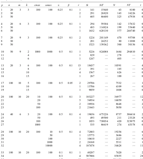
The experiments were designed to evaluate the performance of the algorithm as: (i) dimensions in-crease, (ii) k increases, (iii) cmax increases, (iv)
umaxincreases, (v) increases and (vi)increases. The results are reported in Table 1.As may be seen it is very dicult to make conclusions about the
relation between ; ; cmax; umax and the
di-culty of the problems. Obviously the problems are more dicult to solve as dimensions increase. The non-multiparametric 0 –1-MK problem is NP-hard
Table 1
Computational experiencea
p n m k cmax umax r Si SiT N NT t tT
1 20 3 3 100 100 0.25 0.1 1 141 15840 63 8100 0.09 3.69
2 30 2 291 26820 143 16226 0.11 7.22
3 50 1 605 86600 325 47938 0.11 16.98
4 20 6 3 100 100 0.25 0.1 1 294 59304 142 37632 0.12 14.51
5 30 1 483 114824 199 55440 0.12 18.99
6 50 1 1632 620130 577 246740 0.25 82.72
7 20 9 3 100 100 0.25 0.1 2 1224 201149 470 95708 0.18 34.11
8 30 1 201 24252 80 11088 0.04 4.45
9 50 1 1523 139362 500 50156 0.19 17.14
10 50 9 2 1000 1000 0.5 0.1 1 5226 824088 1684 294810 0.66 92.21
11 4 1 829 — 278 — 0.09 —
12 6 1 1247 — 403 — 0.17 —
13 20 3 6 100 100 0.5 0.1 13 18437 — 10591 — 4.17 —
14 8 2 391 — 185 — 0.15 —
15 10 4 1567 — 626 — 0.32 —
16 15 1 267 — 100 — 0.10 —
17 100 10 5 100 100 0.5 0.05 2 29706 — 7532 — 1.43 —
18 10 1 13706 — 4109 — 0.89 —
19 15 1 9059 — 1808 — 0.65 —
20 100 10 20 10 100 0.5 0.1 3 183227 — 36977 — 12.33 —
21 20 5 54934 — 16059 — 5.61 —
22 50 2 38936 — 8648 — 2.89 —
23 100 2 21643 — 5050 — 1.68 —
24 40 6 3 20 100 0.5 0.1 4 19656 675226 8737 306414 2.79 63.78
25 50 1 493 49500 211 23328 0.06 9.87
26 100 1 1053 730034 420 323075 0.13 69.74
27 1000 1 535 86619 274 45378 0.09 17.14
28 100 10 20 100 10 0.5 0.1 4 72803 — 19256 — 6.55 —
29 50 1 15775 — 3686 — 1.16 —
30 100 1 10610 — 2227 — 0.84 —
31 1000 2 26168 — 5511 — 1.87 —
32 10000 4 187478 — 34628 — 11.15 —
33 100 10 20 100 100 0.1 0.1 1 40287 — 7420 — 2.70 —
34 0.3 4 507806 — 85855 — 28.49 —
35 0.7 15 439616 — 224623 — 30.45 —
36 0.7 6 26271 — 7512 — 1.76 —
37 100 10 20 100 100 0.5 0.05 1 10581 — 2054 — 0.97 —
38 0.15 7 414200 — 93377 — 31.74 —
39 0.20 3 45316 — 9726 — 3.31 —
aNote:p: an index to identify the problem;k: the cardinality of; r: the number of ‘QL-problems’ solved in order to complete the multiparametric analysis;Si: the number of simplex iterations computed to solveQL(1); : : : ; QL(r)andT(2); : : : ; T(r);SiT: the number of simplex iterations computed to solveP(A) for allA∈S(without the multiparametric algorithm); N: the number of nodes generated by the branch and bound algorithm to solveQL(1); : : : ; QL(r)andT(2); : : : ; T(r);NT: the number of nodes generated by the branch and bound algorithm to solveP(A) for allA∈S (without the multiparametric algorithm);t: the CPU-time (seconds) to solveQL(1); : : : ; QL(r)and
with the solved problems. It is obvious that our algo-rithm was much better than solving all the members that dene the multiparametric problem, which is in general a very expensive or impossible task if the car-dinality ofS is large enough (this pattern of analysis was used by Holm and Klein [5]). The symbol ‘−’ in the columns ‘SiT’, ‘NT’ and ‘tT’ (see the prob-lems 11 until 23 and 26 until 39) means that it was impossible to solve P(A) for all A∈S without the multiparametric algorithm because the cardinality of
S is large (from 1080 members ofS corresponding to the problem 17 until millions of members for some of the problems). We are at present performing exper-iments with other kinds of problems before making ‘denitive’ conclusions.
In non-parametric ILP a signicant eort is directed towards the design of special purpose algorithms for problems with particular structures. It is reasonable then to think that a next step should be the design of specialized multiparametric algorithms. The multi-parametric algorithm turns out to be, from this point of view, a general methodology and problemsQL(r)
andT(r)would be solved with specialized algorithms associated to the structure of the problemsP(A).
Acknowledgements
The nancial assistance by CDCH-UCV (project 03.13.3602.95) made the research upon which this
paper is based possible and is gratefully acknowl-edged. We also thank the referees for their helpful comments.
References
[1] B. Bank, R. Mandel, Parametric integer optimization, Math. Res. 39 (1988) 1–138.
[2] A. Crema, A contraction algorithm for the multiparametric integer linear programming problem, European J. Oper. Res. 101 (1997) 130–139.
[3] B. Gavish, H. Pirkul, Ecient algorithms for solving multiconstraint zero-one knapsack problems to optimality, Math. Programming 31 (1) (1985) 78–105.
[4] A.M. Georion, R. Nauss, Parametric and postoptimality analysis in integer linear programming, Management Sci. 23 (1977) 453–466.
[5] S. Holm, D. Klein, Three methods for post-optimal analysis in integer linear programming, Math. Programming Study 21 (1984) 97–109.
[6] L. Jenkins, Parametric mixed integer programming: an application to solid waste management, Management Sci. 28 (1982) 1270–1284.
[7] L. Jenkins, Using parametric integer programming to plan the mix of an air transport eet, INFOR 25 (1987) 117–135. [8] L. Jenkins, Parametric methods in integer linear programming,
Ann. Oper. Res. 27 (1990) 77–96.