School Dropout Rates
Lorraine Dearden
Carl Emmerson
Christine Frayne
Costas Meghir
a b s t r a c t
This paper evaluates a United Kingdom pilot study designed to test whether a means-tested conditional cash transfer paid to 16- to 18-year-olds for staying in full-time education is an effective way of reducing the proportion of school dropouts. The transfer’s impact is substantial: In the first year, full-time education participation rates increase by around 4.5 percentage points while the proportion receiving two years of education increases by around 6.7 percentage points. Those receiving the full payment have the largest initial increase in participation and some evidence is found suggesting that part of the effect can be explained by liquidity constraints.
1. Introduction
Education has been at the center of policies intended to promote growth both in the developing world and in wealthier countries. It is seen as a key
Lorraine Dearden is a professor at the Institute for Fiscal Studies, London, and the Institute of Education, University of London. Carl Emmerson is a researcher at the Institute for Fiscal Studies, London. Christine Frayne is a researcher for the European Commission, Brussels, Belgium. Costas Meghir is a professor at the Institute for Fiscal Studies and Department of Economics, University College London. The authors are thankful to an anonymous referee, Josh Angrist, Erich Battistin, Richard Blundell, Susan Dynarski, Emla Fitzsimons, Alissa Goodman, James Heckman, Caroline Hoxby, Steven Rifkin, and Barbara Sianesi for useful comments on earlier versions of this paper. They are also indebted to their evaluation colleagues Karl Ashworth, Sue McGuire, and Sue Middleton from the Centre for Research in Social Policy and Stephen Finch from the National Centre for Social Research for their support and advice. The authors also received invaluable advice and comments from John Elliott and Ganka Mueller from the former U.K. Department for Education and Skills (DfES), which funded the evaluation. Costas Meghir thanks the Economic and Social Research Council (ESRC) for funding under the Professorial Fellowship RES-051-27-0204. The usual disclaimer applies. An earlier version of this paper appeared as ‘‘Education Subsidies and School Drop-out Rates’’ (Dearden et al.2005).The data used in this article can be obtained beginning May 2010 through April 2013 from Carl Emmerson, Institute for Fiscal Studies, 7 Ridgmount Street, London, WC1E 7AE, UK (e-mail: cemmerson@ifs.org.uk).
½Submitted March 2007; accepted July 2008
ISSN 022-166X E-ISSN 1548-8004Ó2009 by the Board of Regents of the University of Wisconsin System
to development and to the ability of a country to keep up with the fast-moving tech-nological change.1 The recent increase in the returns to education in the United States2 and the United Kingdom3 has reinforced this view. Education is also seen as a way for individuals to escape poverty and welfare (and possibly crime) depen-dency, and this perception has motivated numerous policies worldwide that promote education as a long-run solution to these problems.
The most recent figures show just 76 percent of 25- to 34-year-olds with upper-secondary education in the United Kingdom as of 2006, which is 11 percentage points lower than the corresponding figure for the United States despite continuing problems with dropout rates in the United States, particularly U. S. cities.4
There has been worldwide focus on school dropout rates and a number of policies have been devised to help reduce them. One of the key policy changes in most OECD countries after the Second World War was to introduce free secondary school educa-tion and to increase the compulsory school-leaving age. The timing and pace of these reforms varied tremendously across countries, and in the United States the most im-portant reforms actually occurred before the Second World War.5In the United King-dom, fees for state secondary schools were abolished by the Education Act 1944 (the Butler Act) and the compulsory school-leaving age was increased from 14 to 15 in 1946 and then from 15 to 16 in 1974, where it remains today. In the United States today, the compulsory school-leaving age ranges from 16 to 18;6for the remaining 29 OECD countries, it ranges from 14 to 18.7
Making secondary education free and increasing the compulsory school-leaving age had an effect on school dropout and completion rates, and a number of these re-forms have been analyzed in previous research.8In recent years, a number of coun-tries, both developed and developing, have introduced means-tested conditional grants in an attempt to encourage students to stay in school, rather than simply rais-ing the compulsory school-leavrais-ing age. Conditional cash transfer (CCT) programs have become an important policy option that may well become a permanent feature
1. See, among many others, Benhabib and Spiegel (1994), Krueger and Lindahl (2001), and Vandenbuss che, Aghion, and Meghir (2006).
2. See Juhn, Murphy, and Pierce (1993). 3. See Gosling, Machin, and Meghir (2000).
4. See Table A1.2a, page 43 of OECD (2008). In the United States, students may drop out of school if they have reached the age set in their state’s law for the end of compulsory schooling, which ranges between 16 and 18, but dropouts are not considered to have completed school and no certificate or award is issued at this stage. The U. S. status dropout rate is currently 9.3 percent (see Lairdet al.(2008) Table 6), but the methods for calculating official graduation and dropout rates have been challenged recently in a number of studies and the true figure is likely to be closer to 25 percent—see, for example, Heckman and LaFontaine (2007).
5. See Goldin (1999).
6. Compulsory schooling ends by law at age 16 in 30 states, at age 17 in nine states, and at age 18 in 11 states plus the District of Columbia (see U. S. Department of Education, International Affairs Staff (2005), page13).
7. See Table C.2.1, page 343 of OECD (2008).
in a number of countries. Examples include PROGRESA in Mexico9and Familias en Accio´n in Colombia.10Indeed, such programs have now started in about 20 develop-ing countries worldwide and their scope often extends beyond education outcomes.11 The interest in these programs extends beyond developing countries. A CCT sys-tem has been in operation in Australia since 198812and the Opportunity NYC pro-gram is now being piloted in New York.13In the United Kingdom, a CCT program focused on participation in full-time education——the Education Maintenance Al-lowance (EMA)—has been rolled out on a national basis since September 2004. The EMA is a means-tested program that subsidizes children to remain in school for up to two years beyond the statutory age in the United Kingdom.
The results reported in this paper are based on data from the first cohort of the EMA pilot study, which started in 1999 in a number of areas in England and pre-ceded the national rollout. The target population was pupils who completed their last year of compulsory education (Year 11) in the summer of 1999.14Estimating the im-pact of this program provides valuable information on whether such CCTs, which effectively reduce the cost of education, actually reduce school dropout rates, which at present are the central policy concern.15As such, the results can help guide policy and provide new evidence on the importance of financial incentives in shaping edu-cation choices.
Evidence on the impact of the opportunity cost of education can be found in the literature on education choice: Willis and Rosen (1979), and more recently Heckman, Lochner, and Taber (1999) and Todd and Wolpin (2003), are examples of education choice models that allow for the opportunity cost of education measured as lost earnings.16 Some of the existing direct evidence on the importance of upfront monetary incentives for school participation comes from the PROGRESA experi-ment in Mexico17and from the Familias en Accio´n program in Colombia.18Both
9. See Schultz (2004) and Attanasio, Meghir, and Santiago (2007). 10. See Attanasioet al.(2006).
11. See, for example, Rawlings and Rubio (2005). 12. See Dearden and Heath (1996).
13. See the press release associated with the launch of this program, at http://www.nyc.gov/html/om/html/ 2008a/pr102-08.html.
14. The U. K. government announced on 6 November 2007 that, from 2015, all children will have to re-main in some form of education or training until the age of 18. This policy will run alongside EMAs—see Department for Children, Schools, and Families (2007).
15. With respect to dropping out at 16, following the GCSE qualification which is obtained at that age, the then Minister for Lifelong Learning, Margaret Hodge, stated in Parliament:ÔThe real challenge is to in-crease the number of young people achieving two A-levels. That comes under our schools agenda—our 14 to 19 agenda. A particular problem is the haemorrhaging of young people, who achieve five A to Cs at GCSE level and then do not stay on to do further education full timeÕ(House of Commons Hansard Debatesfor 5 July 2001, column 391). A survey of government policy by Johnson (2004) also highlights this concern.
16. Todd and Wolpin (2003) estimate a model of educational choice and fertility using the control villages from the PROGRESA experiment in Mexico. They then validate their model by testing whether it is capable of predicting the outcomes induced by the experiment. Meghir (1996) estimates the incentive effect of wages on education in Thailand. A 10 percent increase in the wage, which represents an increase in the opportunity cost of schooling, reduces school participation by children on average by 1 percent. His results are described in Tzannatos (2003).
programs establish significant and large effects for 10- to 17-year-olds, but in a very different context from the pilot study examined here.19
In the work presented here, the impact of the EMA is found to be quite substan-tial, especially for those who receive the maximum payment. The CCT increases the initial education participation of eligible males by five percentage points and of el-igible females by four percentage points. In the second year, the CCT increases the proportion staying in full-time education for two years by 7.4 percentage points for eligible males and 5.9 percentage points for eligible females, suggesting that the ef-fect of the policy is to increase not only initial participation but also retention within full-time education. The initial effects are largest for those who receive the maxi-mum payment. It is estimated that around two-thirds of individuals who stayed in education were drawn from inactivity rather than paid work. The effect of the EMA is found to be largest for children with lower levels of prior educational achievement.
Beyond estimating the effects of incentives on education participation, another key issue concerns understanding the mechanism by which subsidies operate. A CCT such as the EMA changes the opportunity cost of education. Thus, from an indi-vidual’s perspective, even if it is optimal not to participate under the prepolicy envi-ronment, it may become optimal to do so postpolicy. The main mechanism that motivates policy, and indeed the presumption of policymakers, has been that low le-vels of education participation are due to financial constraints rather than being the outcome of an informed choice in an unconstrained environment.20The desirability of a CCT in this case would be much greater because it could improve efficiency.
To say something about this, the impact of the CCT on those living in owner-occupied housing is compared with the impact on those living in rented accommo-dation. The parents of the former are unlikely to be liquidity constrained because they are relatively more likely to have access to either financial assets or credit, not least because it is relatively straightforward for them to borrow against the house; whether they are willing to provide the funds to their children, of course, is another matter.21A larger (9.1 percentage point) and statistically significant impact of the policy is found on participation in education among those in rented accommodation compared with a smaller (3.8 percentage point) and not statistically significant im-pact on those in owner-occupied accommodation. However, the 5.3 percentage point
19. Interestingly, Attanasio, Meghir, and Santiago (2007) show the importance of direct evidence and dem-onstrate that the implied monetary incentives provided by a CCT can have much larger effects than those induced by equivalent changes in labour market wages. Other related papers include Dynarski (2003), who examines the impact of incentives for college attendance and completion in the United States, Angrist and Lavy (forthcoming), who use a randomised experiment to assess the sensitivity to monetary incentives for obtaining a high school graduation certificate in Israel, and Angrist, Lang, and Oreopoulos (2006), who use a randomised trial at a Canadian university to examine the impact of increased financial incentives, in-creased nonfinancial support, and both inin-creased financial and nonfinancial support on educational out-comes.
20. ÔWe recognise that for some people there are financial barriers to participating in education, particularly for those from lower income households’ (http://info.emasys1.dfes.gov.uk/control.asp?region¼partners& page¼general).
difference between these two estimates is not statistically different from zero (p-value ¼ 12 percent). Therefore the extent to which the impact of the policy is due to credit constraints, rather than an unconstrained price effect, remains unclear. The paper proceeds as follows. In Section II, the program and its variants and the data used to evaluate the program are described. In Section III, the evaluation meth-odology is discussed. The results are discussed in Section IV along with some robust-ness checks, while concluding remarks are offered in Section V.
II. Background and Data
The EMA pilots were launched in September 1999 in 15 out of the 150 local education authorities (LEAs)22 in England. The scheme paid a means-tested benefit to 16- to 18-year-olds who remained in full-time education after Year 11,23when education ceases to be compulsory (at 16 years of age, approximately). The benefit could be claimed for up to two years (or three for young people with spe-cial educational needs) and could be used to attend any form of full-time post-16 ed-ucation, whether academic or vocational. In this paper, the effects of the EMA on individuals who first became eligible for it in September 1999 are considered.24
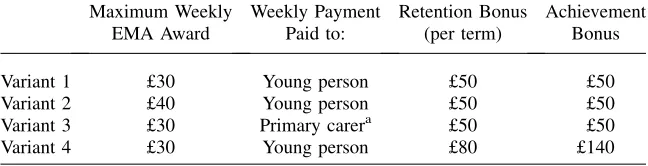
Four different variants of the EMA were piloted and these are outlined in Table 1. The basic EMA (Variant 1) was piloted in eight urban areas and one rural area. Var-iants 2, 3, and 4 were all piloted in two urban areas. In each area, the maximum EMA weekly payment (£30 or £40, which was disregarded for the purposes of both income tax and welfare payments) could be received by young people whose parents’ incomes were £13,000 or below.25 The benefit was tapered linearly for family incomes between £13,000 and £30,000, with those from families earning £30,000 re-ceiving £5 per week. No payment was made for families with income in excess of £30,000. In addition, at the end of a term of regular attendance, the child would re-ceive a nonmeans-tested retention bonus (£50 or £80).26The children also received an achievement bonus on successful completion of their course examination. To put these amounts in context, the median net wage among those who opted for full-time work in the sample was £100 per week. Thus the maximum eligibility for the EMA, depending on the variant, replaces around a third of posttax earnings.
The program was announced in the spring of 1999, just before the end of the school year, and the lateness of the announcement means that it could not have
22.ÔLocal education authorities’ is the term for school districts in the United Kingdom.
23. The U. K. compulsory schooling system is based on 12 years: age 4 (Reception) through to age 16 (Year 11). Participation at ages 17 and 18 (Year 12 and Year 13) is currently voluntary but is also provided free at the point of use in state institutions and is generally necessary for immediate entry into higher ed-ucation.
24. Data are also available from a second cohort, who became eligible for the payment from September 2000. These are not included in the analysis as there is a chance that the academic outcomes in Year 11 of this cohort may have been influenced by the announcement of the program, whereas this is not so for the first cohort because of the timing of the announcement. Only urban areas are considered, as it was only in these areas that all four variants were piloted. Full results for all cohorts and rural areas are available from the authors.
impacted on a child’s Year 11 examination results.27The data used to evaluate the program are based on initial face-to-face interviews with both the parents and the children and on followup annual telephone interviews with the children. The data set was constructed so as to include both eligible and ineligible individuals in pilot and control areas. The data in this paper are from nine urban pilot LEAs, which were selected by the government on the basis of having relatively high levels of depriva-tion, low participation rates in post-16 educadepriva-tion, and low levels of attainment in Year 11 examinations, and nine urban control LEAs, which were selected by the authors of this paper on the basis of having similar participation rates in full-time education in the recent past (both unconditionally and conditional on observed back-ground characteristics of the young person and their parents) and, as far as possible, being geographically close to a pilot area.28A map of England showing the location and proximity of the nine urban pilot and nine urban control areas used in this study is shown in Appendix 1.
The first interview was conducted at the beginning of the school year in which the CCT became available. Respondents were informed that the purpose of the survey was to investigate the destinations of 16- to 19-year-olds after they had finished compulsory schooling, with the same survey instrument used in both pilot and con-trol areas. The proportions of the initially selected sample that yielded usable data were very similar in the pilot and control areas (54.6 percent and 56.4 percent
Table 1
The Four Variants of the EMA
Maximum Weekly EMA Award
Weekly Payment Paid to:
Retention Bonus (per term)
Achievement Bonus
Variant 1 £30 Young person £50 £50
Variant 2 £40 Young person £50 £50
Variant 3 £30 Primary carera £50 £50
Variant 4 £30 Young person £80 £140
a. Usually the mother.
respectively). In the following year, the same students (but not parents) were fol-lowed up using a telephone interview. Attrition between the first and second inter-views is discussed in Section IV.B and Appendix 4.
In addition to information on the child’s current economic activity, the data set contains a wealth of variables relating to family income (which is used to estimate whether the child would be eligible for the EMA were they to reside in an EMA area and continue in full-time education), family background (such as parents’ economic activity, occupation, and education), childhood events (such as ill health and mobil-ity), and prior school achievement. Administrative data on the quality of schooling in the child’s neighborhood and other measures of neighborhood quality measured prior to the introduction of the EMA were also collected.29
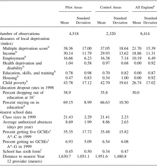
Table 2 provides some prereform neighborhood statistics for the pilot and control areas, while Appendix 2 provides definitions of each of the neighborhood variables used in the analysis.30Larger values of these indices point to a greater level of dep-rivation. For the sake of comparison, the average indices and their standard deviation for the whole of England are also shown. Based on this information, it is clear that the pilots and controls are in more deprived areas and remarkably close to each other relative to the overall variation in England. The control areas were selected on the basis of similar socioeconomic characteristics, and of similar levels and trends of ed-ucation participation for the 16–18 age group. As can be seen from Table 2, the char-acteristics of the treatment and control areas are very similar indeed, with pilot areas tending to be slightly more disadvantaged. Indeed, the (proxy for the) aggregate non-school-participation rate prereform is just less than three percentage points higher in the pilot areas than in the control areas. However, some of the differences between pilot and control areas are statistically significant. This highlights the importance of appropriately weighting the control group, because if these prereform differences are not taken into account, it is likely that the impact of the EMA on participation in ed-ucation would be underestimated.
As explained in Section III, the evaluation methodology is based on the assump-tion of selecassump-tion on observables and uses matching methods. Thus to control for the small differences between pilot and control areas, observed individual-level data from the survey as well as the administrative and local-area data are used. The var-iables used include individual-based characteristics on prior achievement, household income, parental occupation and education, household composition, and ethnicity; they also include childhood variables on early health problems, early childcare and grandparental inputs, special needs, and geographic mobility in early life. Pub-licly available data on the prereform quality of the child’s nearest Year 11 state school31 and distance to the nearest Year 12 state educational provider (post-16
Table 2
Prereform Neighborhood Characteristics of Pilot and Control Areas
Pilot Areas Control Areas All Englanda
Mean
Number of observations 4,518 2,320 8,414
Measures of local deprivation (index)
Multiple deprivation scoreb 38.36 17.00 37.05 18.64 21.70 15.39
Incomeb 30.14 11.79 29.93 13.62 18.86 11.31
Employmentb 16.66 6.23 16.38 7.14 10.19 6.49
Health deprivation and disabilityb
1.04 0.58 0.97 0.68 0.00 0.92
Education, skills, and trainingb 0.78 0.98 0.70 0.82 0.00 0.87
Housingb 0.47 0.83 0.34 1.00 0.00 0.92
Child povertyb 43.78 17.12 42.70 19.61 26.74 17.02
Education dropout rates in 1998
Class sizes in 1999 21.43 2.29 21.41 2.23
Average authorized absences
School has sixth formf 0.45 0.50 0.34 0.47
Distance to nearest Year 12 provider (meters)
1,630.7 1,051.1 1,951.6 1,480.8
a. The all-England data are calculated on the basis of ward-level data (small subdivisions of municipalities). There are 8,414 wards in England.
b. A higher score indicates a higher incidence of deprivation. Scores across different measures are not comparable. c. These data are taken from official LEA-based calculations of 16-year-old stay-on rates in 1998 (Depart-ment for Education and Skills 2005), weighted by the sample populations. (Weighting is necessary, as in two of the control LEAs, half as many individuals as in the other control LEAs were sampled.) d. These data are calculated by looking at the number of 17-, 18-, and 19-year-olds in receipt of Child Ben-efit divided by the number of 13-, 14-, and 15-year-olds receiving the benBen-efit in the local area (ward). Child Benefit is payable for all children under 16 and all those over 16 in secondary education. It has nearly 100 percent takeup. As very few 19-year-olds are in secondary——rather than tertiary—education, this figure is an underestimate (by about a third) of the proportion of young people staying in postcompulsory education and should be understood as a proxy for this figure.
e. GCSE exams are taken in the last year of compulsory education (Year 11) and are graded A* to G. The government has a target for at least 60 percent of 16-year-olds nationwide, and at least 30 percent of pupils in all schools, to achieve five GCSEs at grades A* to C by 2008.
education) have also been controlled for.32The means of the remaining variables used in the analysis are provided in Appendix 3.
III. The Evaluation Methodology
The outcome of interest in this paper is full-time participation in postcompulsory schooling, which is Years 12 and 13. The focus is on the impact of financial incentives on the entire target population—that is, the population of those fully or partially eligible for the CCT as well as the ineligible population (see further discussion in Section IV). In each case, the outcomes are compared relative to an ap-propriate control group.
Although the treatment and control areas are very well matched, the distribution of characteristics is not identical, as would be expected if a large-scale randomization had taken place; some of the differences are statistically significant, albeit small. To allow for the fact that this was not going to be a randomized experiment, the panel data were designed to include a large array of individual and local-area characteris-tics. These should control for any relevant differences in the treatment and control areas before the program was introduced, thus making the assumption of selection on observables and the matching approach credible. Conditional on the observable characteristics, it is assumed that the assignment to treatment is random.33
To estimate the impact of the program on first-year outcomes, three mutually exclu-sive outcomes of interest are defined: full-time education, work, and not in education, employment, or training (NEET). To do this, a demographic group of interest is taken— for example, boys whose family income implies eligibility for a full EMA award were they to live in an EMA pilot area and participate in full-time education. Using data from this group only, a probit model is used to estimate the propensity score— that is, the probability of an individual residing in an EMA pilot area as opposed to residing in an EMA control area, given their observed characteristics. Based on this estimated propensity score, common support across treatment and control observa-tions is checked for. Because of the way the data collection was designed, in practice there are no problems of common support and only a handful of observations are dropped (see the sample sizes in Tables 3 and 4).34The impact is then estimated using kernel-based propensity score matching,35a multinomial probit, and a linear regres-sion model. These are all estimated on the same sample that satisfies the common-support conditions. In the multinomial probit and linear regression models, individual characteristics (discussed in the previous section and listed in Appendix 3), a dummy variable for whether they reside in an EMA pilot area, and interactions between this
32. A number of studies have shown that distance to school is an important determinant of educational decisions (Card 1995 and 1999).
33. See Rosenbaum and Rubin (1983) and Heckman, Ichimura, and Todd (1997).
34. See Rosenbaum and Rubin (1983) for the role of the propensity score and Heckman, Ichimura, and Todd (1997) for the importance of ensuring common support.
dummy variable and all of the other individual characteristics are included. These models are therefore called fully interacted multinomial probit and fully interacted OLS (ordinary least squares) respectively. They produce a set of heterogeneous effects of the policy, similar to the propensity score matching approach. The averages of these heterogeneous effects with respect to the distribution of characteristics for those living in the EMA pilot areas are reported and the results are interpreted as the estimated impact of treatment on the treated. The three models (propensity score matching, fully interacted multinomial probit, and fully interacted OLS) produce almost identical esti-mates of the average impact of the EMA on those who were treated.
Using the second wave of data, estimates of the impact of the EMA on being in full-time education for two years, one year, or no years past the compulsory school-leaving age are calculated. The estimates are produced using propensity score matching as well as a fully interacted ordered probit, fully interacted multinomial probit, and fully interacted linear regression. Again, all models produce almost iden-tical point estimates of the average impact of the EMA on those who were treated. The only difference between the different estimation procedures is the precision of the estimates. Hence, for the remainder of the paper, the fully interacted linear regres-sion approach is used as it is the easiest to implement and gives the most precise results.36The characteristics used include variables relating to family income and back-ground, childhood events (such as ill health and mobility), and prior school achieve-ment, which are all described in Appendix 3, as well as administrative data on the quality of schooling in the child’s neighborhood, other measures of neighborhood qual-ity, and performance at the school level measured prior to the introduction of the EMA. As a final step, some sensitivity analysis is also carried out. In one experiment, ag-gregate school participation data for 16-year-olds including eligible and ineligible pupils are used because aggregate statistics do not measure outcomes for eligible pupils alone.37In the second experiment, the change in school participation between the young person and their next oldest sibling in pilot and control areas is examined, con-trolling for a number of characteristics. The reasons that this variable is not included in the main evaluation methods are that not all children have older siblings and that the time-varying covariates measured, including income, relate to the date of the survey—-that is, when the younger sibling was deciding whether to continue in education or drop out. Nevertheless, these sensitivity analyses confirm the results found with matching. In all cases, the standard errors allow for clustering at the LEA level, which is the unit of treatment. For the linear regression, analytical standard errors are used. For pro-pensity score matching, the fully interacted multinomial probit, and the fully interacted ordered probit models, standard errors are calculated using the block bootstrap.38
36. Note that most of the regressors are discrete and a number of interactions are included. This means that the OLS approach is close to being nonparametric discrete choice by estimating probabilities within cells. Obviously, not all possible interactions were included (there would be far too many), but the results imply that the parametric restrictions imposed are not restrictive. This is clearly demonstrated by comparing to the propensity score method. See the work of Blundell, Dearden, and Sianesi (2005) on this issue. 37. See Department for Education and Skills (2005).
IV. The Results
A. Impact of the EMA on Year 12 Destinations
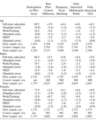
Table 3 shows estimates of the impact of the EMA (overall and by sex) on young people’s initial decisions to remain in full-time education, to move into employment or training, or to be NEET. The table compares the results obtained when one uses the kernel-based propensity score matching technique, fully interacted multinomial probit, and fully interacted linear regression as well as those obtained by a simple comparison of means.
The EMA has had a positive and significant effect on postcompulsory education participation among eligible young people. The overall estimate is around 4.5 per-centage points39from a baseline of 64.7 percent in the matched sample of controls.40 The third and fifth rows of the table show that, as a result of the policy, inactivity declined by three percentage points and work by 1.5 percentage points. These point estimates indicate that a large proportion of the increased school participation orig-inates from those who are otherwise not working, although this finding should be taken with some caution, given the standard errors. This result is important because it shows that, to a large extent, the policy is displacing individuals not from paid work but from financially unproductive activities, thus implying an overall lower fi-nancial cost of providing this incentive to education. This does raise the issue of the quality of individuals attracted to education by the CCT, since they seem to be largely those with little opportunity cost. However, as shown later, they tend to stay in full-time education for the whole two years of the CCT. Moreover, given the reg-ulated nature of the education institutions they have to attend, one can hypothesize they are receiving valuable training. Ultimately, however, this can only be evaluated using eventual labor market outcomes, which are not available for this pilot study.
The effects are larger for males, who have lower participation rates, than for females. However, the difference is not significant at conventional levels.
B. Impact of the EMA in the Second Year (Year 13)
So far, the analysis has concentrated on the impact of the EMA on initial destinations in Year 12, the first postcompulsory year. However, the EMA is available for two years. Thus an important question is whether the impact of the EMA persists in the second year, significantly altering the entire path post-16. Education (whether academic or vocational) at Years 12 and 13 typically consists of courses lasting two years. It is therefore interesting to see whether individuals, having sampled
39. This is the average of the three estimates, and corresponds to the fully interacted OLS estimate. To avoid confusion, only the results of the fully interacted linear regression (OLS) model are reported in all the text that follows.
postcompulsory schooling as a result of the EMA, may have subsequently decided to drop out before Year 13. To answer this question, concentration turns to individ-uals observed for a second year. For this group, the impact of the EMA on staying in
Table 3
Impact of the EMA on Year 12 Destinations of Eligibles
Participation
Full-time education 69.2 +3.9 +4.4 +4.6 +4.5
(Standard error) (0.8) (1.4) (1.4) (1.8) (1.3)
Work/Training 16.4 –0.4 –1.7 –1.6 –1.5
(Standard error) (0.6) (1.1) (1.3) (1.1) (1.2)
NEET 14.5 –3.5 –2.7 –3.0 –3.0
(Standard error) (0.6) (1.1) (1.2) (1.3) (0.8)
Pilot sample size 3,524 3,524 3,518 3,518 3,518
Control sample size n/a 1,791 1,791 1,791 1,791
Total sample size 3,524 5,315 5,309 5,309 5,309
Males
Full-time education 66.4 +5.3 +4.8 +4.6 +5.0
(Standard error) (1.1) (2.0) (2.1) (2.5) (2.0)
Work/Training 19.7 –1.5 –2.9 –2.3 –2.5
(Standard error) (1.0) (1.6) (1.9) (1.7) (2.0)
NEET 13.9 –3.8 –1.8 –2.3 –2.4
(Standard error) (0.8) (1.5) (1.5) (1.8) (1.4)
Pilot sample size 1,753 1,753 1,747 1,747 1,747
Control sample size n/a 900 900 900 900
Total sample size 1,753 2,653 2,647 2,647 2,647
Females
Full-time education 71.9 +2.5 +4.1 +4.6 +4.0
(Standard error) (1.1) (1.9) (2.0) (2.5) (1.7)
Work/Training 13.0 +0.7 –0.5 –0.9 –0.4
(Standard error) (0.8) (1.4) (1.7) (1.3) (1.4)
NEET 15.1 –3.2 –3.6 –3.7 –3.6
(Standard error) (0.9) (1.5) (1.8) (2.0) (0.9)
Pilot sample size 1,771 1,771 1,771 1,771 1,771
Control sample size n/a 891 891 891 891
Total sample size 1,771 2,662 2,662 2,662 2,662
full-time education for two years, one year, or no years (in other words, leaving school at the minimum school-leaving age) is assessed.41
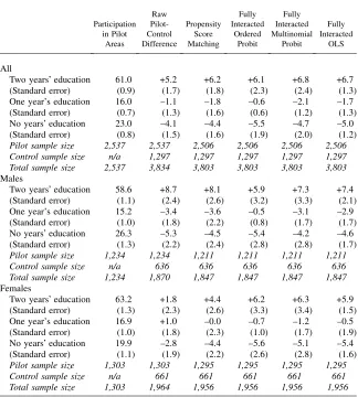
Table 4
Impact of the EMA on Number of Years of Postcompulsory Full-Time Education by Year 13 among Eligibles
Two yearsÕeducation 61.0 +5.2 +6.2 +6.1 +6.8 +6.7
(Standard error) (0.9) (1.7) (1.8) (2.3) (2.4) (1.3)
One year’s education 16.0 –1.1 –1.8 –0.6 –2.1 –1.7
(Standard error) (0.7) (1.3) (1.6) (0.6) (1.2) (1.3)
No yearsÕeducation 23.0 –4.1 –4.4 –5.5 –4.7 –5.0
(Standard error) (0.8) (1.5) (1.6) (1.9) (2.0) (1.2)
Pilot sample size 2,537 2,537 2,506 2,506 2,506 2,506
Control sample size n/a 1,297 1,297 1,297 1,297 1,297
Total sample size 2,537 3,834 3,803 3,803 3,803 3,803
Males
Two yearsÕeducation 58.6 +8.7 +8.1 +5.9 +7.3 +7.4
(Standard error) (1.1) (2.4) (2.6) (3.2) (3.3) (2.1)
One year’s education 15.2 –3.4 –3.6 –0.5 –3.1 –2.9
(Standard error) (1.0) (1.8) (2.2) (0.8) (1.7) (1.7)
No yearsÕeducation 26.3 –5.3 –4.5 –5.4 –4.2 –4.6
(Standard error) (1.3) (2.2) (2.4) (2.8) (2.8) (1.7)
Pilot sample size 1,234 1,234 1,211 1,211 1,211 1,211
Control sample size n/a 636 636 636 636 636
Total sample size 1,234 1,870 1,847 1,847 1,847 1,847
Females
Two yearsÕeducation 63.2 +1.8 +4.4 +6.2 +6.3 +5.9
(Standard error) (1.3) (2.3) (2.6) (3.3) (3.4) (1.5)
One year’s education 16.9 +1.0 –0.0 –0.7 –1.2 –0.5
(Standard error) (1.0) (1.8) (2.3) (1.0) (1.7) (1.9)
No yearsÕeducation 19.9 –2.8 –4.4 –5.6 –5.1 –5.4
(Standard error) (1.1) (1.9) (2.2) (2.6) (2.8) (1.6)
Pilot sample size 1,303 1,303 1,295 1,295 1,295 1,295
Control sample size n/a 661 661 661 661 661
Total sample size 1,303 1,964 1,956 1,956 1,956 1,956
Notes: See Notes to Table 3.
When considering whether the policy has led to longer-term increases in partic-ipation, the second wave of data for the cohort is used. However, there has been some attrition: About 25 percent of the original sample was lost in the followup. Appendix 4 shows that the likelihood of remaining in the sample is higher for those with incomes that would make them eligible for the EMA relative to the rest. How-ever, the pattern of attrition is the same for the treatment and control areas, possibly implying that attrition has mainly changed the overall population composition rather than led to biases for the population being considered. Appendix 4 reports the results of running a probit on the determinants of attrition. This shows that those who come from families earning less than £13,000 per annum (that is, those in the pilot and control groups who are defined as fully eligible) are slightly less likely to drop out of the panel but there is no difference conditional on this eligi-bility between pilot and control areas. These results suggest that attrition was not directly related to the EMA. When the impact of the EMA in the first year is rees-timated using only the sample of those who do not drop out of the panel, very sim-ilar estimates of the overall impact of the EMA on full-time education participation are obtained.42Whilst this is reassuring, it is also clear that the distribution of ob-served characteristics has changed as a result of attrition in the second wave. In particular, the individuals who did not drop out of the sample tended to originate from a relatively advantaged family background (see Appendix 4) and were more likely to be in school in Wave 1 of the data. In this sense, the population used to look at the longer-term outcomes is different from the one used to look at the shorter-term outcomes. However, it should be stressed that issues relating to the impact of attrition are only relevant when one looks at the longer-term effects of the program.
Table 4 shows the impact of the EMA based on the division of the population into the three mutually exclusive groups described above: two years of full-time educa-tion, one year of full-time educaeduca-tion, and no years of full-time education after the minimum school-leaving age. Again, all of the estimation methods give reassuringly similar results. The discussion refers to the last column of results, which is based on the fully interacted linear regression technique. The important conclusion that comes from the table is that the EMA has been particularly effective in increasing the pro-portion of students staying in school in both Year 12 and Year 13, and thus it is shown to have long-term effects. The estimated impact is slightly larger than for the first year (although again not significantly so). This result is important because it indicates that those drawn into education due to the EMA are committed to it. They do not just sample it only to find that it is not for them and drop out a few months later. A formal test of the impact of the EMA on retention (the proportion of those in full-time education in Year 12 who stay on in Year 13) finds that the EMA increased retention rates by 4.1 percentage points from 77.6 percent to 81.7 percent. This effect is statistically significant at conventional levels.43
42. For males, 5.1 percentage points with a standard error of 1.8, compared to the estimate of 5.0 percent-age points for the full sample. For females, 4.3 percentpercent-age points with a standard error of 1.5, compared to the estimate of 4.0 percentage points for the full sample.
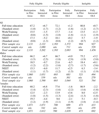
C. Impact of the EMA in Year 12, by Eligibility Group
In this section, the impact of the EMA is estimated separately for those who are esti-mated to be potentially eligible for a full award and those who are estiesti-mated to be po-tentially eligible for only a fraction because their parents have an income higher than £13,000. The impacts may be different for the two groups for a number of conflicting reasons. First, if the CCT award is lower, it is likely to have a smaller effect. Second, the individuals who receive a lower CCT do so because they come from a better-off background; this may make them more likely to go to school in the first place and thus may also affect their sensitivity to upfront monetary incentives. With this policy de-sign, it is not possible to distinguish one effect from the other. Thus, Table 5 distin-guishes between full eligibility, partial eligibility, and ineligibility to see whether the impact of the EMA differs according to whether a person was fully or only partially eligible and to see whether there were any spillovers to those in the ineligible group. Just over 47 percent of individuals are estimated to have been eligible for the max-imum EMA payment, around 31 percent eligible for partial payment, and 22 percent not eligible. All eligible individuals were entitled to the full bonuses.
Among those who were estimated to be eligible for a full EMA award, the EMA increased full-time education participation in Year 12 by 6.7 percentage points. For those estimated to be eligible for only a partial award, the corresponding figure is 1.2 percentage points (and not statistically significant at conventional levels). The p-value for their difference is 2.5 percent. Thus it is possible to say with reasonable confidence that the response of those fully eligible is larger than the response of those on the taper. A survey of education policy in England by Johnson (2004) has high-lighted that one of the key aims of policies such as the EMA is to improve post-compulsory staying-on rates for children from deprived social backgrounds. The combination of a more generous payment and possibly their greater responsiveness to the payment points to a success of the policy in this dimension.44
Similarly, for ineligible individuals, the overall effect is very small (+0.7 percent-age points) and not statistically significant at conventional levels, indicating that the spillover effects, at least in the short run, are not important.
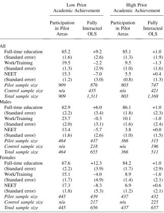
D. Does the Impact Vary by Prior Academic Achievement?
It has already been shown that the EMA has its largest impact on children from rela-tively lower-income families who are able to qualify for the maximum award (Table 5). Another key question is whether children with low prior academic achievement can be encouraged to stay in school longer, possibly improving their skills before labor market entry. Thus, in Table 6, results split into low and high prior educational achievement are presented, where the sample is those eligible for a full EMA award only.45The
44. According to pages 177–8 of Johnson (2004),ÔThe U. K. has a relatively low staying-on rate in full time education after age 16. Given high returns this is, perhaps, surprising and probably economically in-efficient. Given very substantial differences in staying-on rates by social background, it is also of concern from an equity point of viewÕ.
EMA seems to affect primarily those with low prior educational achievement. How-ever, this is perhaps not so surprising, given that the postcompulsory school-participa-tion rate is much higher for those with high prior achievement. It does point out, however, that the increase in participation comes primarily from the lower ability group and is consistent with the earlier results showing that a large proportion of the increase in participation comes from those who would not otherwise be in paid work (Table 3 and Table 5). This may raise the question of whether the returns to
Table 5
Impact of the EMA on Year 12 Destinations: All Young People by Eligibility
Fully Eligible Partially Eligible Ineligible
Full-time education 67.2 +6.7 72.1 +1.2 80.8 +0.7
(Standard error) (1.0) (1.7) (1.2) (1.8) (1.2) (1.7)
Work/Training 15.5 –1.5 17.7 –1.4 13.5 +1.3
(Standard error) (0.8) (1.5) (1.0) (1.8) (1.1) (1.9)
NEET 17.3 –5.2 10.1 +0.2 5.7 –1.9
(Standard error) (0.8) (1.3) (0.8) (1.2) (0.7) (1.2)
Pilot sample size 2,131 2,122 1,393 1,372 994 927
Control sample size n/a 1,080 n/a 711 n/a 529
Total sample size 2,131 3,202 1,393 2,083 994 1,456
Males
Full-time education 66.2 +6.7 66.7 +4.0 75.2 +3.2
(Standard error) (1.5) (2.5) (1.8) (2.9) (1.9) (3.0)
Work/Training 18.5 –0.7 21.6 –6.5 18.4 +0.1
(Standard error) (1.2) (2.2) (1.6) (2.7) (1.7) (3.6)
NEET 15.3 –6.0 11.7 +2.5 6.3 –3.4
(Standard error) (1.1) (1.7) (1.2) (1.5) (1.1) (1.9)
Pilot sample size 1,060 1,051 693 683 521 494
Control sample size n/a 539 n/a 361 n/a 270
Total sample size 1,060 1,590 693 1,044 521 764
Females
Full-time education 68.2 +6.8 77.6 –1.6 86.9 –2.2
(Standard error) (1.4) (2.3) (1.6) (2.2) (1.6) (1.8)
Work/Training 12.5 –2.3 13.9 +3.6 8.0 +2.5
(Standard error) (1.0) (1.5) (1.3) (2.4) (1.3) (1.8)
NEET 19.3 –4.4 8.6 –2.1 5.1 –0.3
(Standard error) (1.2) (1.9) (1.1) (1.9) (1.0) (1.4)
Pilot sample size 1,071 1,071 700 689 473 433
Control sample size n/a 541 n/a 350 n/a 259
Total sample size 1,071 1,612 700 1,039 473 692
Table 6
Impact of the EMA on Year 12 Destinations of Those Fully Eligible for the EMA, by Prior Academic Achievement
Low Prior Academic Achievement
High Prior Academic Achievement
Participation in Pilot
Areas
Fully Interacted
OLS
Participation in Pilot
Areas
Fully Interacted
OLS
All
Full-time education 65.2 +9.2 85.1 +1.0
(Standard error) (1.6) (2.6) (1.3) (1.9)
Work/Training 19.5 –2.2 9.5 –1.3
(Standard error) (1.3) (2.9) (1.0) (1.6)
NEET 15.3 –7.0 5.5 +0.4
(Standard error) (1.2) (3.0) (0.8) (1.3)
Pilot sample size 909 876 803 747
Control sample size n/a 435 n/a 421
Total sample size 909 1,311 803 1,168
Males
Full-time education 62.9 +6.0 86.1 +1.0
(Standard error) (2.2) (3.4) (1.8) (2.3)
Work/Training 23.7 –0.3 10.1 –1.0
(Standard error) (2.0) (3.1) (1.6) (2.4)
NEET 13.4 –5.7 3.8 +0.0
(Standard error) (1.6) (2.6) (1.0) (1.5)
Pilot sample size 464 437 366 315
Control sample size n/a 218 n/a 196
Total sample size 464 655 366 511
Females
Full-time education 67.6 +12.3 84.2 +1.0
(Standard error) (2.2) (3.9) (1.7) (2.9)
Work/Training 15.1 –4.0 8.9 –1.6
(Standard error) (1.7) (4.9) (1.4) (2.1)
NEET 17.3 –8.3 6.9 +0.6
(Standard error) (1.8) (5.3) (1.2) (2.1)
Pilot sample size 445 439 437 432
Control sample size n/a 217 n/a 225
Total sample size 445 656 437 657
education for this group are sufficiently large to justify the program, an issue that can-not be resolved with the available data.
E. Credit Constraints?
The estimates imply that the EMA has a relatively large impact on the education par-ticipation decisions in both Year 12 and Year 13, with a substantial effect on com-pleting two years of postcompulsory schooling. A key question, which is directly relevant for understanding the way the policy works and for evaluating its merits, is whether the estimated effect is due to liquidity constraints or is simply the re-sponse to the ‘‘distorted incentive’’ induced by the CCT. In general, most pupils have no direct access to savings. Most pupils need to borrow to fund education, if only because living expenses have to be covered, and, in practice, such funding typically comes from the parents since it is unlikely that a young person of 16 will have access to capital markets. Part of the parental funding will be motivated by straight altruism: If the parents value the child’s utility, they will be willing to fund education that will improve the lifecycle welfare of the child,46although the amount they fund will not normally be the optimal level from the perspective of the child. If the child can com-mit to repay some of the funds, the parents may be willing to advance even more. Otherwise, the child will be effectively liquidity constrained. In addition, parents with little or no assets and low income may in fact be unable to provide adequate funding, possibly being liquidity constrained themselves, leading the child to work instead of attending school. This is the primary concern of policymakers.
Thus, the policy may lead to the increases in participation in two alternative ways. One is a simple price distortion: By subsidizing education, its market price has been artificially lowered and children who would not otherwise attend school do so. This can be shown to be the case in a household that is altruistically linked or if the child is acting as an individual.47In this case, their private returns to education (net of costs) might be low. The other additional mechanism is that the CCT alleviates a li-quidity constraint and children obtain more education now that a market distortion against education has been (at least partially) corrected. Under the null of no liquid-ity constraints, the child has access to all the funding required for their optimal level of schooling.
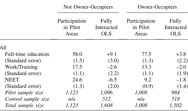
To get a handle on this issue, a long tradition in the consumption literature48is followed. The sample is split by assets, the idea being that those with assets are not liquidity constrained. The measure of assets used is house ownership, since fam-ilies that own a house are relatively more likely to have access to financial assets or credit—not least as it would be relatively straightforward for them to release equity by borrowing against the house. Under the null hypothesis, it is assumed that once the plethora of socioeconomic characteristics, ability, and local variables have been controlled for, house ownership is not correlated with the perceived costs of, or returns to, schooling.
46. See Becker (1991).
Given this assumption, a comparison is made between the impact of the policy on those living in an owner-occupied house and the impact on those living in rented ac-commodation (prepolicy). The key assumption here is that house ownership in itself does not lead to different responses to financial incentives, other than because it implies different access to funds.49Under the null, those in rented accommodation will react in the same way as those in owner-occupied housing because in both cases they were able to obtain the optimal amount of schooling prepolicy. Postpolicy, the price of education is distorted and this affects both groups in the same way. Under the alternative, however, those in rented accommodation will have two reasons to in-crease education: First, they will now have the opportunity to fund education when before they could not; second, they will face the price distortion. Overall, those in rented accommodation should respond more to the CCT.
The results of this test are presented in Table 7. The point estimate of the impact of a full EMA award is 9.1 percentage points for nonowner-occupiers, while the esti-mated impact for owner-occupiers is substantially smaller (3.8 percentage points). The difference between the two coefficients is significant at the 12 percent level. Therefore, while the point estimates indicate the importance of liquidity constraints, the standard error of the difference in the effects between the two groups is a bit too large for a firm conclusion.
This hypothesis of liquidity constraints has implications for policy. Were the differ-ence in outcomes due to the presdiffer-ence of credit constraints, then the policy would have
Table 7
Impact of the EMA on Year 12 Destinations of Those Fully Eligible for the EMA, by Housing Tenure
Not Owner-Occupiers Owner-Occupiers
Participation in Pilot
Areas
Fully Interacted
OLS
Participation in Pilot
Areas
Fully Interacted
OLS
All
Full-time education 58.0 +9.1 77.5 +3.8
(Standard error) (1.5) (3.0) (1.3) (2.2)
Work/Training 17.5 –2.6 13.3 –2.0
(Standard error) (1.1) (2.2) (1.1) (1.9)
NEET 24.6 –6.5 9.2 –1.8
(Standard error) (1.3) (2.0) (0.9) (1.4)
Pilot sample size 1,123 1,096 1,008 984
Control sample size n/a 512 n/a 518
Total sample size 1,123 1,608 1,008 1,502
Notes: See Notes to Table 3.
much stronger grounds for support, as it would suggest that lack of finances leads to undereducation of children from low-income families. Irrespective of the presence of credit constraints, the policy could be more effectively targeted on asset holdings (although not without introducing further long-run distortions).
The liquidity constraints story does not sit comfortably with the fact that most of the increase in schooling comes from a reduction in unpaid activities rather than paid work. This does highlight the price distortion idea as a stronger possibility. However, the fact that the low-asset people respond much more may also point to an alternative interpretation:50Some young people are discounting the future returns from education too heavily and therefore placing relatively too much weight on the upfront costs of remaining in school. If these individuals were disproportionately more likely to reside in rented rather than owner-occupied accommodation, then it might also explain why those in the former group respond more strongly to the EMA and, potentially, why (if anything) these young people seem to have been drawn from the group not in educa-tion, employment, or training as opposed to being drawn from those in paid work.
F. Sensitivity Analysis
As a final robustness check, the results from two sensitivity tests are presented, both using a difference-in-differences approach. In the first case, the impact is estimated using aggregate school participation data. In the second, the impact is estimated by comparing the behavior of children in the survey with that of their next oldest sibling who was too old to be eligible for the EMA.
1. Aggregate Data
This section presents simple difference-in-differences estimates based on aggregate school participation data for 16-year-olds. Three postpolicy periods are compared to the one prepolicy period (1998) where there is a complete set of data. In reading these results, note that the proportion of fully eligible individuals is about 47 percent. Including those partly eligible (that is, on the taper) increases the proportion to 78 percent. Under the assumption that the policy had no effect on ineligible individuals, the estimated effect on all individuals needs to be multiplied by 1.3 in order to esti-mate the impact of the EMA on those eligible for it.
The three difference-in-differences estimates for 1999, 2000, and 2001 are respec-tively 2.7, 2.3, and 4.7 percentage points, always with 1998 as the baseline.51 Mul-tiplying these estimates by 1.3 gives effects of 3.5, 3.0, and 6.1 percentage points respectively, which are remarkably close to the effect obtained from the individual data of 4.5 percentage points (Table 3), and certainly within the 95 percent confi-dence interval.
2. Using Older Siblings
An alternative approach, which allows one to focus more closely on the group of in-terest and at the same time to control for characteristics as in the main analysis, is to
50. See Oreopoulos (2007).
use difference-in-differences, with the next oldest sibling of the children in the pilot and control areas as a comparison group. This allows examination of the change in participation between the current cohort and the older siblings in the pilot and control areas, controlling for observed characteristics. A full set of cohort and area dummies are included. The estimated effect of the EMA using this approach is 8.4 percentage points (with a standard error of 2.6), which is larger than the effect reported above. The difference is not significant at conventional levels.52 The smaller sample has made the estimate less precise, but it offers support for the significant effect of the EMA.
Finally, successive difference-in-differences across siblings reaching the statutory school-leaving age before the period when the policy was in place are carried out. In all previous periods, this placebo ‘‘effect’’ is not statistically significant. In the final period, when the policy was in place, a positive and statistically significant effect is obtained, again corroborating and strengthening the results.
G. A Back-of-the-Envelope Cost–Benefit Calculation
If the strong impact of the EMA is due to liquidity constraints, then even in the ab-sence of any externalities to education, a positive welfare effect of the policy could be expected. However, this is hard to measure because there is no measure of the in-dividual costs of education, and nor is it easy to measure the distortionary effects of raising funds for the CCT. Nevertheless, the results of a simple, back-of-the-envelope calculation are presented.
The EMA increased the percentage of individuals from income-eligible families completing two years of postcompulsory education by 6.7 percentage points, from 54.3 percent to 61.0 percent. In the first year (second year), one-third (two-thirds) of this increase was from individuals who would otherwise have been in paid em-ployment.53This means that those brought into education would need to experience a real increase in future earnings of 6.2 percent as a result of the additional two years of education for the program to break even, allowing for the opportunity cost of ed-ucation.54Allowing £3,000 for the extra annual cost of educating those who stay on in secondary education55increases the required return to education for the two years to 7.7 percent. Research into the returns from staying on in postcompulsory education suggests that the returns are in fact 11 percent for males and 18 percent
52. The standard error allows for clustering at the family level.
53. Results for the split between paid work and NEET for the second year are available on request. 54. To do this calculation, the rate of return to education,r, that solves+1
t¼0 found, whereEMAtis the annual average CCT allowing for the fact that not all those eligible receive a full
award (this average is estimated to be £900 a year—£25 a week for 30 weeks plus £150 in bonuses) andpis the proportion in full-time education eligible for the EMA (estimated to be 75.2 percent).atis the proportion drawn from paid employment at timet, which is estimated to be one-third fort¼0 (Year 12) and two-thirds fort¼1 (Year 13).lis the increase in participation in education (estimated to be 6.7 percentage points from Table 4).Ctis the marginal cost of those brought into education as a result of the EMA andwtrepresents the
estimated life-cycle wage profile based on the 2002–03Family Resources Survey. Real growth in future wages of 2 percent a year is assumed.Ris the discount rate and is assumed to be 3 percent, which is the recommen-ded discount rate in the U. K. HM TreasuryGreen Book(http://greenbook.treasury.gov.uk/).
for females.56There may well be other benefits of the policy: The government might value the redistribution to lower-income families with children; infra-marginal indi-viduals may reduce hours of work and increase effort put into education; there may be crime reductions. Many of these benefits are hard to evaluate but they should not be discounted without further research.57
V. Conclusions
Conditional cash transfers have become very popular as a way of im-proving participation in schools. One such policy intervention, and probably unique in scope in a rich industrialized country, is the Education Maintenance Allowance in the United Kingdom. Despite a steady increase, the participation in education follow-ing completion of compulsory schoolfollow-ing in the United Kfollow-ingdom remained relatively low before its introduction. Since September 2004, the EMA program has been rolled out nationally.
The results in this paper imply that the scope for affecting education decisions us-ing CCTs can be substantial. More specifically, they imply that the EMA has signif-icantly raised the stay-on rates past the age of 16. The initial impact is around 4.5 percentage points, with no effect on ineligibles. Taking into account that this was a time when the labor market was particularly buoyant, these seem to be quite large effects, although they were achieved with a replacement rate of 33–40 percent of av-erage net earnings for the age group.
The results also suggest that the impact of the EMA on participation actually increases in the following year. This result is important because it suggests that those who are induced into extra education do not find the courses unexpectedly difficult or uninteresting and are willing to stay for the full two years of the program. Impor-tantly, about two-thirds of the initial increase in school participation is due to a de-cline in inactivity rather than in work. This reduces the implicit costs of the program because the forgone earnings for these individuals are zero. However, this may also mean that the program is attracting those with few other opportunities, as also dem-onstrated by the fact that the largest effect is among those with low prior achieve-ment. The key policy question here is the extent to which this extra education is valuable to them. If the main mechanism by which the policy works is by alleviating liquidity constraints, then it would reinforce the view that those attracted into educa-tion by this policy would enjoy positive net returns. Among those eligible for a full award, the point estimate of the effect of the policy is larger for renters than for owner-occupiers. While this is consistent with some families facing credit constraints, the difference in the estimated impact of the policy is not statistically dif-ferent from zero at conventional levels of significance. Therefore the extent to which the impact of the policy is due to credit constraints, rather than an unconstrained price effect, remains unclear.
56. See Dearden, McGranahan, and Sianesi (2004).
The returns realized by those induced into staying on by the CCTs are not known. Furthermore, there is little evidence on how these returns and the future supply of educated workers may change now that the program has been rolled out nationally. This, of course, depends on many factors, not least the nature of the production func-tion. These are all important research and policy questions that need to be investi-gated in the future.
Appendix 1
Map of England Showing Location and Proximity of the Nine Urban Pilot and Nine Urban Control Areas Used in This Paper
Appendix 2
Indicators Used in Each Deprivation Score
Income Adults in Income Support households (DSS) for 1998
Children in Income Support households (DSS) for 1998 Adults in Income-Based Jobseeker’s Allowance households
(DSS) for 1998
Children in Income-Based Jobseeker’s Allowance households (DSS) for 1998
Adults in Family Credit households (DSS) for 1999 Children in Family Credit households (DSS) for 1999 Adults in Disability Working Allowance households (DSS)
for 1999
Children in Disability Working Allowance households (DSS) for 1999
Nonearning, non-Income-Support pensioner, and disabled Council Tax Benefit recipients (DSS) for 1998 apportioned to wards
Employment Unemployment claimant counts (JUVOS, ONS) average of
May 1998, August 1998, November 1998, and February 1999
People out of work but in TEC-delivered government-supported training (DfEE)
People aged 18–24 on New Deal options (Employment Survey)
Incapacity Benefit recipients aged 16–59 (DSS) for 1998 Severe Disablement Allowance claimants aged 16–59 (DSS)
for 1999 Health deprivation
and disability
Comparative mortality ratios for males and females at ages under 65; district-level figures for 1997 and 1998 applied to constituent wards (ONS)
People receiving Attendance Allowance or Disability Living Allowance (DSS) in 1998 as a proportion of all people Proportion of people of working age (16–59) receiving
Incapacity Benefit or Severe Disablement Allowance (DSS) for 1998 and 1999 respectively
Age- and sex-standardized ratio of limiting long-term illness (1991 Census)
Proportion of births of low birth weight (<2,500g) for 1993–97 (ONS)
Education, skills, and training
Working-age adults with no qualifications (three yearsÕ aggregated LFS data at district level, modeled to ward level) for 1995–98
Children aged 16 and over who are not in full-time education (Child Benefit data—DSS) for 1999
Appendix 2 (continued)
Proportions of 17- to 19-year-old population who have not successfully applied for higher education (UCAS data) for 1997 and 1998
Key Stage 2 primary school performance data (DfEE, converted to ward-level estimates) for 1998
Primary school children with English as an additional language (DfEE) for 1998
Absenteeism at primary level (all absences, not just unauthorized) (DfEE) for 1998
Housing Homeless households in temporary accommodation (Local
Authority HIP Returns) for 1997–98 Household overcrowding (1991 Census)
Poor private sector housing (modeled from 1996 English House Condition Survey and RESIDATA)
Geographical access to services
Access to a post office (General Post Office Counters) for April 1998
Access to food shops (Data Consultancy) for 1998
Access to a GP (NHS, BMA, and Scottish Health Service) for October 1997
Access to a primary school (DfEE) for 1999
Child poverty Percentage of children that live in families that claim means-tested benefits (Income Support, Income-Based Jobseeker’s Allowance, Family Credit, and Disability Working Allowance)
Source: Department of the Environment, Transport, and the Regions (2001).
Appendix 3
Sample Means
Whole Sample
Pilot Areas
Control Areas
Pilot area 0.661 1.000 0.000
Fully eligible for the EMA 0.470 0.472 0.466
Partially eligible for the EMA 0.308 0.308 0.306
Not eligible for the EMA 0.223 0.220 0.228
In full-time education Year 12 0.709 0.717 0.694
In work Year 12 0.156 0.157 0.154
Characteristics used in matching
Male 0.504 0.503 0.504
Weekly family income 389.01 387.50 391.95
Appendix 3 (continued)
Family receives means-tested benefit 0.263 0.268 0.253
Mother and father figure present 0.623 0.626 0.617
Father figure present 0.753 0.753 0.753
Father’s age (¼0 if absent) 30.096 30.301 29.696
Mother’s age 39.859 39.867 39.843
Owner-occupier 0.693 0.686 0.709
Council or Housing Association 0.253 0.266 0.226
Has statemented special needs 0.092 0.093 0.090
Mother has A levels or higher 0.245 0.237 0.259
Mother has O levels or equivalent 0.246 0.245 0.247
Father has A levels or higher 0.221 0.220 0.223
Father has O levels or equivalent 0.171 0.168 0.177
Father manager or professional 0.166 0.163 0.172
Father clerical or similar 0.243 0.246 0.238
Mother manager or professional 0.129 0.121 0.144
Mother clerical or similar 0.294 0.300 0.282
Father variables missing 0.363 0.362 0.366
One or two parents in work when born 0.831 0.825 0.843
Attended two primary schools 0.254 0.256 0.251
Attended more than two primary schools
0.076 0.077 0.073
Received childcare as a child 0.911 0.915 0.903
One set of grandparents around
Ill between 0 and 1 0.223 0.225 0.219
Number of older siblings 0.941 0.928 0.968
Number of younger siblings 0.975 0.979 0.968
Older sibling educated to 18 0.291 0.286 0.299
White 0.896 0.892 0.903
Father in full-time work 0.503 0.504 0.502
Father in part-time work 0.021 0.019 0.025
Mother in full-time work 0.335 0.327 0.350
Mother in part-time work 0.309 0.312 0.304
Math GCSE score 4.233 4.232 4.235
English GCSE score 3.810 3.798 3.834
GCSE score missing 0.129 0.131 0.126
Appendix 4
Probability of Attrition between Wave 1 and Wave 2
Marginal Effect Standard Error
Partially eligible for the EMA 20.002 0.024
Fully eligible for the EMA 20.039 0.015
Pilot area +0.005 0.012
Male +0.019 0.011
Weekly family income +0.000 0.000
Family receives means-tested benefit 20.014 0.017
Mother and father figure present 20.015 0.032
Father figure present 20.028 0.021
Owner-occupier 20.085 0.025
Council or Housing Association 20.031 0.023
Has statemented special needs 20.001 0.018
Mother’s age 20.002 0.001
Father’s age 20.001 0.001
Mother has A levels or higher +0.001 0.017
Mother has O levels or equivalent +0.001 0.014
Father has A levels or higher 20.065 0.018
Father has O levels or equivalent 20.022 0.017
Father manager or professional 20.014 0.021
Father clerical or similar +0.017 0.016
Mother manager or professional 20.029 0.020
Mother clerical or similar 20.014 0.013
Father variables missing 20.015 0.036
One or two parents in work when born 20.011 0.016
Attended two primary schools 20.021 0.012
Attended more than two primary schools +0.030 0.021
Received childcare as a child +0.002 0.019
One set of grandparents around when child
20.008 0.015
Two sets of grandparents around when child
+0.004 0.016
Grandparents provided care when child +0.007 0.012
Ill between 0 and 1 +0.010 0.013
Number of older siblings +0.017 0.006
Number of younger siblings 20.010 0.005
Older sibling educated to 18 20.036 0.013
White 20.020 0.022
Father in full-time work +0.033 0.020
Father in part-time work 20.004 0.039
Mother in full-time work 20.002 0.017
Mother in part-time work 20.030 0.015