SHELLS OF MATRICES IN INDEFINITE INNER PRODUCT SPACES∗
VLADIMIR BOLOTNIKOV†, CHI-KWONG LI† ‡, PATRICK R. MEADE† §,
CHRISTIAN MEHL¶, AND LEIBA RODMAN†
Abstract. The notion of the shell of aHilbert space operator, which is auseful generalization (proposed by Wielandt) of the numerical range, is extended to operators in spaces with an indefinite inner product. For the most part, finite dimensional spaces are considered. Geometric properties of shells (convexity, boundedness, being a subset of a line, etc.) are described, as well as shells of operators in two dimensional indefinite inner product spaces. For normal operators, it is conjectured that the shell is convex and its closure is polyhedral; the conjecture is proved for indefinite inner product spaces of dimension at most three, and for finite dimensional inner product spaces with one positive eigenvalue.
Key words. Indefinite inner products, Numerical range, Shells, Normal matrices.
AMS subject classifications. 15A60, 15A63, 15A57
1. Introduction. LetH ∈Cn×nbe a Hermitian matrix. Define the sesquilinear
form (indefinite inner product) associated withH by
[x, y]H =y∗Hx, x, y∈Cn
,
where y∗ denotes the conjugate transpose of the vector y. For a matrixA ∈Cn×n,
let
WH(A) =
[Av, v]H
[v, v]H : v∈C n
, [v, v]H = 0
⊆C,
(1.1)
and
SH(A) =
[Av, v]H
[v, v]H ,
[Av, Av]H
[v, v]H
: v∈Cn,[v, v]H = 0
⊆C×R.
(1.2)
WhenH =In, these reduce to the (classical)numerical rangeW(A) and the
Davis-Wielandt shell S(A) of the matrix A, which have been studied extensively; see [9, Chapter 1], [3, 4, 10, 2]. These concepts are useful in studying matrices or operators because of the interesting interplay between the algebraic properties of the matrix
A and the geometrical properties of the sets WH(A) and SH(A). For example, the following properties are well known whenH =In; see [9, Chapter 1].
∗Received by the editors on 25 January 2002. Final manuscript accepted on 1 May 2002. Handling
Editor: Ludwig Elsner.
†College of William and Mary, Department of Mathematics, P.O.Box 8795,
Williams-burg, VA 23187-8795 ([email protected], [email protected], [email protected], [email protected]).
‡The research of this author is partially supported by NSF Grant DMS 0071994.
§The research of this author was done as an undergraduate at William and Mary, and was partially
supported by NSF Grant DMS 9988579.
¶Fakult¨at II; Institut f¨ur Mathematik, Technische Universit¨at Berlin, D-10623 Berlin, Germany
The research of this author is partially supported by NSF Grant DMS-9988579.
(1) W(αA+βIn) =αW(A) +{β} for anyα, β∈C.
(2) W(U∗AU) =W(A) for any unitary matrixU.
(3) W(A) is convex.
(4) W(A) ={λ} if and only ifA=λI. (5) W(A)⊆Rif and only ifAis Hermitian.
(6) W(A) is a line segment if and only ifαA+βI is Hermitian for someα, β∈C
withα= 0.
(7) IfAis normal, thenW(A) is the convex hull of the eigenvalues. The converse is true ifn≤4.
Many of these properties have been extended toWH(A) in [14]; see also [11, 12]. The purpose of this paper is to develop corresponding results forSH(A) for a generalH. SinceWH(A) is the image ofSH(A) under the projection (z, r) →z, one expects thatSH(A) can tell more aboutAthanWH(A). In fact, in the classical case, we have the following intriguing result; see [3].
(8) S(A) is a polyhedron, i.e., the convex hull of a finite number of points in
C×R, if and only ifAis normal.
Studying possible extensions of this result for generalSH(A), and additional geometric properties ofSH(A) for matricesA that are normal with respect to the sesquilinear form [·,·], is one of the main objectives of our study.
The paper is organized as follows. In Section 2, we give some preliminary def-initions and notations; we also describe some general approaches for our study and some related concepts. In Section 3, we prove results relating algebraic properties of
Aand geometrical properties of the set
SH+(A) =
[Av, v]H
[v, v]H ,
[Av, Av]H
[v, v]H
: v∈Cn,[v, v]H >0
,
closely related to SH(A). In Sections 4 and 5, we study whether one can extend property (8) to the general case. It is shown by examples that SH+(A) need not be closed nor bounded, even ifAis assumed to be normal with respect to [·,·]H, or in shortH–normal; see (2.5) for the definition. We prove that for anH–normalAin the following two cases: (a)n≤3; (b)H is invertible with only one positive eigenvalue, the setSH+(A) is convex and its closure is either the whole ofC×R∼=R
1×3 or the intersection of finitely many closed halfspaces. We conjecture that this property is valid for allH–normal operators in finite dimensional indefinite inner product spaces. In Section 6, several results of previous sections are extended to operators on infinite dimensional inner product spaces. Section 7 contains a Maple program that we used in the initial stage of our project to compute examples of shells, and to formulate and check conjectures.
Throughout the paper, we denote byH a fixedn×nHermitian matrix which is not negative semidefinite. In various sections, we may assume additional hypotheses aboutH. We use Conv(S) to denote the convex hull of the setS. For a given matrix (or vector) X, XT and X∗ stand for the transpose and the conjugate transpose,
respectively. Diagonal matrices with entries h1, . . . , hn on the main diagonal are written as diag (h1, . . . , hn). A complex number z is written z = Re(z) +iIm(z), where Re(z) and Im(z) are real. Finally, we denote byR,R+,R+
real numbers, positive real numbers, nonnegative real numbers, and complex numbers, respectively.
2. Preliminaries. Let
S−
H(A) ={([Av, v]H, [Av, Av]H) : v∈C
n,[v, v]H=
−1}
and
SH+(A) ={([Av, v]H, [Av, Av]H) : v∈C
n,[v, v]H= 1
}.
Then
SH(A) =S−
H(A)∪ S + H(A).
We always assume that the set of vectorsvsuch that [v, v]H = 1 (resp., [v, v]H =−1) is not empty when consideringS+
H(A) (resp.,SH−(A)). All the setsSH(A),SH+(A) and
S−
H(A) will be referred to as theDavis-Wielandt shellsofAwith respect toH in our study. SinceS−
H(A) =S +
−H(A), we focus only onS +
H(A). We will often identifyC×R withR1×3 via (a+ib, c) →(a, b, c) in (1.2), and in analogous formulas forS−
H(A) and
S+
H(A). Also, it will be convenient to representS +
H(A) in matrix notation:
SH+(A) =
x∗
HA+A∗H 2
x, x∗
HA−A∗H 2i
x, x∗A∗HAx
: x∈Cn
, x∗Hx= 1
.
If H is invertible, the H-adjoint ofA is denoted byA[∗], which is uniquely defined by the relation
[Au, v] = [u, A[∗]v] u, v∈Cn
(2.1)
and it can be expressed explicitly in terms ofA andH by
A[∗]:=H−1A∗H.
(2.2)
A matrixAis calledH–selfadjoint,H–unitary, orH–normalif
A=A[∗], A[∗]A=In or AA[∗]=A[∗]A,
(2.3)
respectively. In view of (2.2), the three equalities (2.3) are equivalent, respectively, to
HA=A∗H, A∗HA=H or A∗HA=HAH−1A∗H.
(2.4)
In the case when detH = 0, relation (2.1) does not determine a unique H–adjoint of A and of course formula (2.2) does not make sense anymore. However, one can introduceH–selfadjoint andH–unitary matrices using the first two relations in (2.4).
The notion of H–normality introduced in [14] is a little bit more delicate. A matrixA is calledH–normalif
A∗HA=HAH[−1]A∗H,
whereH[−1]denotes the Moore–Penrose pseudoinverse ofH, which is uniquely defined by the conditions
H[−1]HH[−1]=H[−1], HH[−1]H =H, H[−1]H =HH[−1]=P
RangeH,
and wherePRangeH stands for the orthogonal projection onto RangeH.
We start with some useful facts: Proposition 2.1. LetA∈Cn×n.
(a)If r >0 andt∈R, then
SH+(re itA) =
SH+(A)
rcost rsint 0
−rsint rcost 0
0 0 r2
.
(b)If λ∈C, then
S+
H(A+λI) = (Re(λ),Im(λ),|λ| 2) +
S+ H(A)
1 0 λ+λ
0 1 i(λ−λ)
0 0 1
.
(c) LetT be any invertiblen×n matrix. Then
S+
H(A) =S + T∗HT(T−
1AT). (2.6)
Proof. To check (c), just replaceT xbyyin the following chain of equalities:
S+
T∗HT(T− 1AT) =
{(x∗T∗HAT x, x∗T∗A∗HAT x) : x∗T∗HT x= 1}
={(y∗HAy, y∗A∗HAy) : y∗Hy= 1} = S+
H(A).
Statements (a) and (b) follow from the definitions ofSH+(reitA) andS +
H(A+λI) upon simple algebraic manipulations.
Thus, the transformation
(A, H) →(T−1AT, T∗HT)
(2.7)
preserves shells. This transformation also preserves the classes ofH–selfadjoint,H– unitary, andH–normal matrices:
Lemma 2.2. LetH ∈Cn×n be Hermitian and possibly singular and letT ∈Cn×n be invertible. Then A ∈ Cn×n is H–normal (resp., H–selfadjoint, or H–unitary) if and only ifA isH–normal (resp., H–selfadjoint, or H–unitary), whereA=T−1AT
andH =T∗HT.
Proof. We verify the lemma only for theH–normal matrices. First we note that the Moore–Penrose pseudoinverse ofH equals H[−1] =T−1H[−1](T−1)∗. Therefore,
on account of (2.5),
HAH[−1]A∗H =T∗HT T−1AT T−1H[−1](T−1)∗T∗A∗(T−1)∗T∗HT
which completes the proof.
Theorem 2.3. Assume that the positive semidefinite matrixH is singular, and
denote byP the orthogonal projection along the kernel ofH. IfA isH-normal, then
P AP (considered as a linear transformation on (KerH)⊥) is P HP-normal, where
P HP stands for the restriction of H to(KerH)⊥, and
S+
H(A) =S +
P HP(P AP).
Proof. Applying transformation (2.7), we can assume that
A=
A11 A12
A21 A22
and H =
H1 0
0 0
,
whereH1is a positive definite matrix. Then P AP =A11,P HP =H1, andH[−1]=
H−1
1 0
0 0
. Condition (2.5) now givesA12= 0 and
A∗
11H1A11=H1A11H1−1A∗11H1, which means thatP AP isP HP-normal. Finally,
HA=
H1A11 0
0 0
, A∗HA=
A∗
11H1A11 0
0 0
,
and the result follows.
For Hermitian matrices A1, . . . , Ap ∈ Cn×n, we denote by W(A1, . . . , Ap) their
joint numerical range:
W(A1, . . . , Ap) ={(x∗A1x, . . . , x∗Apx)∈Rp : x∈Cn, x∗x= 1}
and byσ(A1, . . . , Ap) theirjoint spectrum:
σ(A1, . . . , Ap) ={(a1, . . . , ap)∈Rp: A1x=a1x, . . . , Apx=apxfor somex= 0}.
The next proposition, which is easy to verify, shows the connection betweenS+ H(A) and the joint numerical range, whose study can be reduced to the 2×2 case by compression.
Proposition 2.4. Let HA = F +iG, where F and G are Hermitian, and
K=A∗HA. Then
SH+(A) =
(a+ib, c) :a, b, c∈R, (a, b, c,1)∈
t>0
t W(F, G , K, H)
,
and
W(F, G , K, H) =
X∈Cn×2, X∗X=I 2
Since the 2×2 case may be used to study the general case, it is useful to have a complete description of this low dimensional case. Recall that a subsetS of a real linear space has affine dimension m if the set S −v0 spans an m−1 dimensional subspace for some (any)v0∈S.
Proposition 2.5. LetA∈C2×2and letmbe the dimension of the real subspace spanned by the set
{H, HA+A∗H, i(HA−A∗H), A∗HA}.
(2.8)
ThenS+
H(A), regarded as a subset of R
1×3, has affine dimensionm
−1. In p articular, if m= 1, then S+
H(A) is a singleton. If m >1, then one of the following conditions
holds.
(a) H is positive definite; m= 2and S+
H(A) is a nondegenerate closed line
seg-ment, equivalently,AisH-normal and not a (complex) scalar multiple of I2;
m= 4 andSH+(A)is an ellipsoid without interior in all other cases.
(b) H = 0is positive semidefinite and singular;m= 4andSH+(A)is a paraboloid without interior.
(c) H is indefinite; m= 2 andSH+(A)is a (closed or open) half line or a whole
line; m= 3 andSH+(A) is a one-component hyperbola with interior, an open
two-dimensional half plane, or a two-dimensional plane; m= 4 and SH+(A)
is a one-component hyperboloid without interior.
Proof. The proposition follows from [13, Theorem 2.1], which describes the joint numerical ranges of ap-tuple of 2×2 Hermitian matrices with respect to a sesquilinear form inC2. We need only to make the following observations that take into account
the special form of the matricesHA+A∗H,i(HA−A∗H), andA∗HA.
(a) By Proposition 2.1, we may assumeH =I2. It is easy to see thatm= 1 if
A=λI,λ∈C,m= 2 ifA=λI and is normal, andm= 4 in all other cases.
(b) Assume that H =
1 0 0 0
, and write A =
a b
c d
. One easily verifies
thatm= 1 ifb= 0, andm= 4 in all other cases.
(c) We assume that H =
1 0 0 −1
, and write A =
a b
c d
. To compute
the dimension m of the span of the set in (2.8), we may assume that a =−d ≥0; otherwise, we may replace A by a matrix of the form µ(A−ηI) for some suitable
µ, η∈C with|µ|= 1. We may further assume thatb ≥0; otherwise replace (H, A)
by (D∗HD, D∗AD) = (H, D∗AD) for a suitable diagonal unitary matrixD. Assume
first thata= 0. Then the four matrices (2.8) take the form
1 0 0 −1
,
0 b−c
b−c 0
,
0 i(b+c)
i(−b−c) 0
,
−|c|2 0 0 b2
.
It is easy to see, using the fact that the complex numbersb−candi(b+c) are linearly independent over R if and only if b2 = |c|2, that m = 2 if b2 =|c|2 and m = 4 if
b2=|c|2. Assume now thata= 0. Then (2.8) takes the form
1 0 0 −1
,
2a b−c
b−c 2a
,
0 i(b+c)
i(−b−c) 0
,
a2− |c|2 a(b+c)
a(b+c) b2
−a2
Ifb+c= 0, then clearlym= 2. If b+c= 0, then
a2
− |c|2 a(b+c)
a(b+c) b2
−a2
+ (−a2+s)
1 0 0 −1
+r
2a b−c
b−c 2a
=
0 a(b+c) +r(b−c)
a(b+c) +r(b−c) 0
,
wherer= (−b2+
|c|2)/(4a),s= (
|c|2+b2)/2. If the complex numbers
a(b+c) +r(b−c) and i(b+c) (2.9)
are linearly independent overR, thenm= 4; otherwise,m= 3. A simple calculation
shows that the complex numbers in (2.9) are linearly independent overRif and only
if 2a=±(b2
− |c|2)/
|b+c|.
3. Geometric properties of shells. In this section we study geometric prop-erties of shells: convexity, degeneracy (being a singleton, or a subset of a line), bound-edness.
We start with the problem of convexity. For the 2×2 case, this can be easily sorted out using the general description of shells of 2×2 matrices in Proposition 2.5. Proposition 3.1. Let A ∈ C2×2. Then SH+(A) is convex if and only if the matricesH,(HA+A∗H), i(HA−A∗H), andA∗HAare linearly dependent.
In general, the shell is not convex, for matrices of size larger than 2: Example 3.2. Let
H=
1 0 0 0 −1 0 0 0 1
, A=
0 0 0 2 0 0 0 0 0
.
ThenHA=F+iG, where
F =
0 1 0 1 0 0 0 0 0
, G=
0 i 0
−i 0 0 0 0 0
, and A∗HA= −
4 0 0 0 0 0 0 0 0
.
Settingx= [x1x2x3]T, we note thatx∗Hx= 1 if and only if|x1|2− |x2|2+|x3|2= 1. A simple calculation shows that
SH+(A) ={(2Re (x1x2),2Im (x1x2),−4|x1| 2) :
|x1|2− |x2|2+|x3|2= 1}.
This set is not convex, for instance if we take the cross-section where−4|x1|2=−16. In this case|x2|2=|x1|2+|x3|2−1≥3, and therefore the cross section ofSH+(A) is
{(2Re (x1x2),2Im (x1x2),−16) : |x2|2≥3}={(q, r,−16) : q2+r2≥48},
Sufficient conditions for convexity are given in the following theorem. Theorem 3.3. LetHA=F+iGbe such thatF, Gare Hermitian. ThenS+
H(A)
is convex if any one of the following two conditions holds.
(a)The four matrices H, F, G, A∗HAare linearly dependent.
(b)n≥3, and the span of{H, F, G, A∗HA} contains a positive definite matrix. Proof. The result follows from [13, Theorem 3.2 (a) and (b)].
We say that a set in Rk is polyhedral if it is the intersection of finitely many
closed half spaces; Rk itself will also be considered a polyhedral set. Clearly, every
polyhedron is a polyhedral set; a polyhedral set is a polyhedron if and only if it is bounded. Also, every polyhedral set is convex.
Theorem 3.4. Let A ∈ Cn×n, K = A∗HA, and HA = F +iG be such that
F and G are Hermitian. Suppose there exists an invertible T such that T∗HT =
diag(h1, . . . , hn),T∗F T = diag(f1, . . . , fn)andT∗GT = diag(g1, . . . , gn). Then
W(F, G , K, H) = Conv{(fj, gj, hj(fj2+gj2), hj) : 1≤j≤n}
is a polyhedron, and thus
S+ H(A) =
(a+ib, c) :a, b, c∈R, (a, b, c,1)∈
t>0
t W(F, G , K, H)
is the intersection of an affine space with a convex polyhedral cone, which is a poly-hedral set.
Proof. The assertion onW(F, G , K, H) is well known; see [1]. The assertion on
S+
H(A) follows readily from Proposition 2.4.
Matrices with degenerate shells are characterized as follows. Theorem 3.5. Let A∈Cn×n. Then:
(a) S+
H(A) is a singleton if and only if the matrix HA is a (complex) scalar
multiple of H.
(b) SH+(A)is a subset of a line if and only ifHA=uH+vGandA∗HA=rH+sG
for some u, v ∈ C, r, s ∈ R, and some Hermitian G which is not a scalar multiple of H; equivalently, the matrices H, HA+A∗H, i(HA−A∗H),
A∗HAspan a two dimensional real subspace. Proof. The result follows from [13, Theorem 3.5]. For boundedness of shells, we have the following result.
Theorem 3.6. The shell SH+(A)is bounded if and only if the kernel of H isA–
invariant (this condition is obviously satisfied if H is invertible) and EITHERH is positive semidefinite ORH is indefinite and there existsα∈Csuch thatHA=αH.
Proof. The “if” part. Applying transformation (2.7), we can assume that
A=
A11 0
A21 A22
, H =
H1 0
0 0
,
whereH1is invertible. Then
which is clearly bounded ifH1is positive definite, or ifH1A11=αH1for someα∈C.
The “only if” part. IfSH+(A) is bounded, then so is the set
WH+(A) ={[Av, v]H :v∈C
n
,[v, v]H = 1}.
The boundedness of WH+(A) is characterized in [11, Theorem 2.3], implying the result.
4. Normality and polyhedral shells: Semidefinite case. The purpose of this section is to study whether Property (8) in Section 1 can be extended to the general case when H is positive semidefinite. First, consider the case when H is positive definite. Without loss of generality, one can assume that H = In. We fix
A∈Cn×n along with its representationA=F +iG, whereF andGare Hermitian
matrices. Furthermore,S+H(A) andSH(A) are the same asW(F, G, A∗A).
Lemma 4.1. If a+ib, a, b ∈ R, is an eigenvalue of A, then (a, b, a2+b2) ∈
W(F, G, A∗A), and the inequalitya2+b2
≤cholds for every(a, b, c)∈W(F, G, A∗A).
Proof. Let U be a unitary matrix, such that U∗AU is of the upper triangular
form witha+iblying in the (1,1) position and letube the first column ofU. Then
(a, b, a2+b2) = (u∗F u, u∗Gu, u∗A∗Au)∈W(F, G, A∗A).
Now, suppose v ∈ Cn is a unit vector such that v∗Av = a+ib, then Av =
(a+ib)v+dw for some d≥0 and some unit vector w∈Cn satisfying v∗w = 0. It
follows thatv∗A∗Av=a2+b2+d2
≥a2+b2.
The following two results have been established in [1].
Lemma 4.2. If(a1, a2, a3)is a vertex point ofW(A1, A2, A3), then(a1, a2, a3)∈
σ(A1, A2, A3).
Corollary 4.3. If W(A1, A2, A3)is a polyhedron, then
W(A1, A2, A3) = Conv (σ(A1, A2, A3)).
The next theorem was essentially proved in [3, 4] using a different approach. Theorem 4.4. Let A=F+iG. The following are equivalent:
(a) W(F, G, A∗A)is a polyhedron in R1×3.
(b) W(F, G, A∗A) = Conv (σ(F, G, A∗A)).
(c) Ais normal.
Proof. Implication (c) ⇒ (a) follows from Theorem 3.4. Implication (a) ⇒ (b) follows readily from Corollary 4.3. To prove implication (b) ⇒ (c), suppose
W(F, G, A∗A) = Conv (σ(F, G, A∗A)). Then W(F, G, A∗A) is a polyhedron. We
claim that every eigenvalue ofAis reducing. Suppose S={aj+ibj : 1≤j≤k}are the distinct eigenvalues ofA. By Lemma 4.1, we have
Conv{(aj, bj, a2j+b 2
j) : 1≤j ≤k} ⊆W(F, G, A∗A)⊆Conv (σ(F, G, A∗A)). Hence Conv{(aj, bj, a2j+bj) : 12 ≤j ≤k}= Conv (σ(F, G, A∗A)). Since the function
f(x, y) =x2+y2is strictly convex onR1×2, and all the points (a
graph, we see that each point (aj, bj, a2j+b2j) is a vertex of the set Conv{(aj, bj, a2j+b2j) : 1≤j ≤k}. By Lemma 4.2, we see that eachaj+ibj is a reducing eigenvalue ofA. HenceA is normal.
IfH is only positive semidefinite, we have the following result, extending Davis’ theorem (statement (8) of Section 1).
Theorem 4.5. Let H ∈ Cn×n be positive semidefinite and singular. Then the following statements are equivalent for A∈Cn×n:
(a) SH+(A) is a polyhedron. (b) SH+(A) is a polyhedral set. (c) A isH-normal.
Proof. (c)⇒(a) follows from Theorem 2.3 and the property (8) of Section 1. (a)
⇒(b) is trivial.
(b)⇒(c). Without loss of generality, we let
H =
Ik 0
0 0
, A=
A11 A12
A21 A22
,
where A11 and A22 are k×k and (n−k)×(n−k), respectively. Arguing by con-tradiction, assume thatA is not H-normal. If A12 = 0, thenA11 is not Ik-normal. On the other hand, SI+k(A11) = S
+
H(A) (cf. the proof of Theorem 2.3), and there-foreSI+k(A11), being a bounded polyhedral set, is a polyhedron, a contradiction with
Theorem 4.4.
Now supposeA12= 0. Lett >5A11, consider the level set
St={v∗(HA)v : v∗Hv= 1, v∗(A∗HA)v=t2},
which coincides with the projection on the first two components of the set
SH+(A)∩ {(x1, x2, t 2)
∈R1×3 : x1, x2∈R}.
SinceA12= 0, there exists w∈Cn−k such thatA12w= 0. Letxbe a unit vector in
Ck. Then there existsν ∈Csuch that A11x+A12(νw)=t.If v=
x νw
∈Cn,
then v∗(HA)v ∈ St. Thus, St = ∅. Clearly, St is a polyhedral set. Using the
Cauchy-Schwartz inequality
|v∗HAv|=|(v∗H)(HAv)| ≤√v∗Hv√v∗A∗HHAv=√v∗Hv√v∗A∗HAv=t
for every v ∈ Cn satisfying v∗HAv ∈ St, we see that the set St is bounded, and
therefore is a convex polygon (with interior).
Let µ =v∗(HA)v be a corner point ofSt. Writingv =
x y
, wherex ∈Ck,
y∈Cn−k, we have
µ=x∗A
We claim that x∗A
12y = 0. Suppose not, i.e., let x∗A12y = 0. We construct a real positive functionδ(θ), whereθ∈(−r, r) for somer >0, such thatδ(0) = 1, and
A11x+A12(eiθδ(θ)y)=t, −r < θ < r,
(4.1)
as follows. Letting x∗A∗
11A12y = u+iw, u, w ∈ R, a calculation shows that δ(θ) satisfies the quadratic equation
(δ(θ))2−1y∗A∗
12A12y+ 2δ(θ) ((cosθ)u−(sinθ)w)−2u= 0. (4.2)
Note thatA12y= 0, becausex∗A12y= 0. SinceA11x+A12y=t >5A11, we see that the product of the roots of the above equation is
−1−2u/A12y2≤ −1 + 2A11x A12y/A12y2≤ −1 + 2A11/(t− A11)<0.
Thus, equation (4.2) always has a positive rootδ(θ) and a negative root. Therefore,
δ(θ) is a differentiable (even analytic) function ofθ. Consider the curve
µ(θ) =x∗A
11x+eiθδ(θ)x∗A12y, −r < θ < r. By (4.1),µ(θ)∈St; alsoµ(0) =µ. Since
lim
θ→0(µ(θ)−µ)/θ= (i+δ
′(0))x∗A
12y,
the line {µ+s(i+δ′(0))x∗A
12y : s ∈ R} is the tangent to the curve µ(θ) at µ, a contradiction with µ being a corner ofSt. Thus,x∗A
12y = 0, and µ belongs to the standard numerical rangeW(A11) ofA11. So,
St= Conv{the corners ofSt} ⊆W(A11). (4.3)
Now, using the hypothesis thatA12 = 0, select x∈Ck, y ∈Cn−k so that x∗x= 1,
x∗A
12y =A12y, and replacing, if necessary,y byµy for some µ > 0 we can also assume thatt=A11x+A12y. Then A12y ≥ t− A11x and since t >5A11, we have
|x∗A
11x+x∗A12y| ≥ |x∗A12y| − |x∗A11x| ≥(t− A11x)− A11>A11. Hence,Stcontainsx∗A11x+x∗A12y, which does not belong toW(A11), a contradic-tion with (4.3).
5. Normality and polyhedral shells: Indefinite Cases. Note that ifH is indefinite,S+
H(A) fails to be a polyhedral set even forH-selfadjoint matrices. Indeed,
ifH =
0 1 1 0
andA=
0 1 0 0
is anH-selfadjoint matrix, then
HA=
0 0 0 1
and A∗HA=
0 0 0 0
Thus, lettingv= (v1, v2)T ∈C2, we have that
SH+(A) ={(|v2|
2, 0, 0) : Re(v
1v2) = 1}={(x,0,0) : x >0}
is an open half line, which is not a polyhedral set. This example also shows that
SH+(A) need not be closed or bounded for an H-normal matrix A. Nonetheless, we have the following conjecture.
Conjecture 5.1. SH+(A) is convex and the closure ofSH+(A)is a polyhedral set
for everyH-normal matrix A.
Conjecture 5.1 is supported by the results of the next four subsections where we explicitly compute shells of particular H-normal matrices. In this context, we will make use of the complete classification ofH-normal matrices for the case whenH is an invertible Hermitian matrix with only one positive eigenvalue. This classification was obtained in [6].
Theorem 5.2. Let H be invertible Hermitian and let H have only one positive
eigenvalue. Furthermore, let X be H-normal. Then there exists an integer m ≥0
and a nonsingular matrix P such that
P−1XP =
X1 0
0 X2
, P∗HP =
H1 0
0 −Im
,
whereX2∈Cm×m is a diagonal matrix form >0, or elseX2 andIm are void, and
the pair (X1, H1)is of one of the following forms:
type 1: X1=λ,H1= 1,λ∈C;
type 2: X1=
λ1 0
0 λ2
,H1=
0 1 1 0
,λ1=λ2;
type 3: X1=
λ z
0 λ
,H1=
0 1 1 0
,λ∈C,|z|= 1;
type 4: X1=
λ z r
0 λ z
0 0 λ
,H1=−
0 0 1 0 1 0 1 0 0
,
whereλ∈Cand either |z|= 1, r∈R,0≤arg(z)< π, orz= 1,r∈iR;
type 5: X1 =
λ cos(φ) sin(φ) 0
0 λ 0 1
0 0 λ 0
0 0 0 λ
, H1 = −
0 0 0 1 0 1 0 0 0 0 1 0 1 0 0 0
, λ ∈ C,
0< φ≤π
2.
Proof. This follows directly from [6, Theorem 2], by consideringX and−H.
5.1. Shells of some specialH-normal matrices. In this subsection, we ex-plicitly compute the shellS+
H(X), whereX andH have one of the following forms:
1)X ∈Cn×nis an upper triangular Toeplitz matrix andH=
1 . .. 1
∈Cn×n.
2) X =
X1 0
0 X2
andH = 1 . .. 1
upper triangular Toeplitz matrices.
It is easy to check that in both cases the matrixX is H-normal. In [7] and [8] it was shown that for a large class ofH-normal matrices a canonical form consisting of blocks of the forms 1) and 2) above can be obtained. (Those H-normal matrices were called block-ToeplitzH-normal matrices in [7]). This and the fact that blocks of the forms 1) and 2) also appear in Theorem 5.2 motivate our interest in these special
H-normal matrices. Before computing the shells, we start with a technical result. Proposition 5.3. Let α1, . . . , αn ∈ R, α1 = 0. Then there exists a vector
v= (v1, . . . , vn)T ∈Cn such that
vnvm+vn−1vm+1+· · ·+vmvn=αm for m= 1, . . . , n (5.1)
if and only ifαn−2k>0 for somek≤ n−21 andaj = 0 forj=n−2k+ 1, . . . , n.
Moreover, in this casev can be chosen real.
Proof. ( ⇒ ): Let l ≥0 be such that αn−l = 0 andαn−j = 0 for j < l. Then (5.1) successively implies vn−j = 0 for j < 2l. Suppose that l = 2k+ 1 is odd, then we havevn=. . .=vn−k= 0. But then (5.1) implies
0 =vnvn−2k−1+· · ·+vn−kvn−k−1+vn−k−1vn−k+· · ·+vn−2kvn=αn−2k−1, i.e., αn−l= 0 which is a contradiction. Thus, l is even, i.e., l = 2k for some integer
k≥0. Then we havevn =. . .=vn−k+1 = 0 and vn−kvn−k =αn−2k. This implies
αn−2k >0.
( ⇐ ): Without loss of generality, we may assume that k = 0. Otherwise, we
have vn = . . . = vn−k+1 = 0 and setting v1 = . . . = vk = 0 and wj = vk+j for
j= 1, . . . , n−2k, equation (5.1) reduces to
wn−2kwm+wn−2k−1wm+1+· · ·+wmwn−2k =αm form= 1, . . . , n−2k, and we can consider the analogous problem with sizen−2kinstead of n. Then we construct the desired vectorv by choosingvn =√αn ∈ Rand computing vm from (5.1) successively as the solution of a linear equation of the form 2vmvn = bm for somebm∈R.
Theorem 5.4. Let x1, . . . , xn∈C,ε=±1, and
H =ε
0 ... 1
1 0
∈Cn×n, and X =
x1 x2 . . . xn
x1 . .. ...
. .. x2
x1 ∈
Cn×n,
(5.2)
an upper triangular Toeplitz matrix. Furthermore, let
˜
xm:=x1xm+x2xm−1+· · ·+xmx1, m= 1, . . . , n,
Xm:= (Re(xm), Im(xm), x˜m), m= 1, . . . , n,
S1:= Span(X2, . . . ,Xn−1), s1:= dim(S1),
S3:= Span(X2, . . . ,Xn−3), s3:= dim(S3),
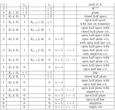
Table 5.1
Classification of shells ofH-normals of the form(5.2)
s1 s3 s5 shell ofX
3 ≤3 ≤3 R1×3
2 Xn∈ S1 ≤2 ≤2 plane
2 Xn∈ S/ 1 2 ≤2 closed half space
2 Xn∈ S/ 1 1 Xn−2∈ S3 ≤1 open half space with line on boundary
2 Xn∈ S/ 1 1 Xn−2∈ S/ 3 1 closed half plane o.b.open half space with
2 Xn∈ S/ 1 1 Xn−2∈ S/ 3 0 n= 6
open half space with open half plane o.b. with open half line o.b.
2 Xn∈ S/ 1 1 Xn−2∈ S/ 3 0 n= 5 ε= 1
open half space with open half plane o.b. with singleton o.b.
2 Xn∈ S/ 1 1 Xn−2∈ S/ 3 0 n= 5 ε=−1 open half space withopen half plane o.b.
2 Xn∈ S/ 1 0 0 n= 4 open half space with open half line o.b.
1 Xn∈ S1 ≤1 ≤1 line
1 Xn∈ S/ 1 1 ≤1 closed half plane
1 Xn∈ S/ 1 0 0 n= 4 open half plane withopen half line o.b.
1 Xn∈ S/ 1 0 0 n= 3 ε= 1 open half plane with singleton o.b. 1 Xn∈ S/ 1 0 0 n= 3 ε=−1 open half plane
0 0 0 n= 2 open half line
0 0 0 n= 1 ε= 1 singleton
0 0 0 n= 1 ε=−1 empty set
Then the shellSH+(X)ofX has the form given by Table 5.1, where “o.b.” means “on
the boundary”. In particular,SH+(X)is convex and its closure is a polyhedral set.
Proof. Letv = (v1, . . . , vn)T ∈Cn be such thatvnv1+vn−1v2+· · ·+v1vn =ε and set
αm=vnvm+· · ·+vmvn, form= 2, . . . , n.
A simple computation shows that
v∗HXv=x
[image:14.595.107.478.181.536.2]Thus,SH+(X) is the set of all points
ε(α1X1+α2X2+· · ·+αnXn),
where α1 := ε, α2, . . . , αn are such that there exists v ∈ Cn such that (5.1) holds. Applying Proposition 5.3 and classifying the shell ofX with respect to the dimensions of the vector spacesS1,S3, andS5, and some other parameters, yields the classification of Table 5.1.
Proposition 5.5. Let α1, . . . , αn, β1, . . . , βn ∈ R. Then there exists a vector
v= (v1, . . . , v2n)T ∈C2n such that
v2nvm+v2n−1vm+1+· · ·+vn+mvn=αm+βmi, m= 1, . . . , n. (5.3)
Proof. Set v2n = v2n−1 = . . . = vn+1 = 1. Then, we determine vn, . . . , v1 successively from (5.3).
Theorem 5.6. Let x1, . . . , x2n∈C,
X1=
x1 x2 . . . xn
x1 . .. ...
. .. x2
x1
, X2=
xn+1 xn+2 . . . x2n
xn+1 . .. ...
. .. xn+2
xn+1
,
upper triangular Toeplitz matrices, and
X =
X1 0
0 X2
, H =
0 1
...
1 0
2n×2n
.
Then the shell S+
H(X) of X is a singleton, a line, a plane, or R 1×3
. In p articular, S+
H(X)is convex and its closure is a polyhedral set.
Proof. Let α1 = 12 and let α2, . . . , αn, β1, . . . , βn ∈ R be arbitrary. By Propo-sition 5.5, there exists a vectorv = (v1, . . . , v2n)T ∈ C2n such that (5.3) holds. In particular, we have
v2nv1+v2n−1v2+· · ·+v1v2n= 1
2+β1i+ 1
2−β1i= 1. A simple computation shows
v∗HXv
= (α1+β1i)x1+· · ·+ (αn+βni)xn+ (α1−β1i)xn+1+· · ·+ (αn−βni)x2n =α1(x1+xn+1) +· · ·+αn(xn+x2n) +β1i(x1−xn+1) +· · ·+βni(xn−x2n),
v∗X∗HXv
where
˜
xm:=x1xn+m+x2xn+m−1+· · ·+xmxn+1 and x˜n+m:= ˜xm, form= 1, . . . , n.
Thus, setting
Xm=
Re(xm+xn+m), Im(xm+xn+m), ˜xm+ ˜xn+m
, m= 1, . . . , n,
Ym=
Im(xn+m−xm), Re(xm−xn+m), i(˜xm−x˜n+m)
, m= 1, . . . , n,
we obtain that
SH+(X) =
1
2X1+α2X2+· · ·+αnXn+β1Y1+· · ·+βnYn: α2, . . . , αn, β1, . . . , βn∈R
.
Hence, the shell of X is a singleton, a line, a plane, orR1×3, depending on the
dimension of the subspace spanned byX2, . . . ,Xn,Y1, . . . ,Yn.
5.2. Shellsof2×2H-normal matrices. The case whenH ∈Cn×nis positive
definite is covered in Theorem 3.1: SH+(A) is a straight line segment, wheneverA is
H–normal. Now we express the coordinates of the vertices of this segment in terms of eigenvalues of the matrixA.
By Lemma 4.2, if (a, b, c) is a vertex ofSH+(A), then
A+A∗
2
=ax,
A−A∗
2i
=bx, A∗Ax=cx
(5.4)
for some nonzerox∈R2. It follows from the first two equalities in (5.4) that
Ax= (a+ib)x, A∗x= (a−ib)x,
(5.5)
and in particular, a+ib is an eigenvalue of A. Since A is H-normal, we have now from (5.5) and the third equality in (5.4)
cx=A∗Ax=A∗(a+ib)x= (a+ib)(a−ib)x= (a2+b2)x
thatc=a2+b2. Therefore, the shell
SH+(A) is a (possibly degenerate) line segment
SH+(A) ={t(a1, b1, a 2
1+b21) + (1−t)(a2, b2, a22+b22) : 0≤t≤1},
where a1+ib1 anda2+ib2 are eigenvalues of A. It can be easily shown that for a fixedH, the shellSH+(A) of anH–normal matrixAis a line segment with vertices on a paraboloid and this paraboloid depends onH and not onA.
for a 2×2H-normal matrixA. This canonical form is a special case of the canonical form in Theorem 5.2. We are then left with the following three types of blocks.
Type 1:
A=
λ1 0
0 λ2
, H =
1 0 0 −1
, λ1, λ2∈C.
In this case, it follows from Proposition 2.5 (see also Theorem 3.4) that S+
H(A) is a closed half line.
Type 2:
A=
λ1 0
0 λ2
, H =
0 1 1 0
, λ1, λ2∈C, λ1=λ2.
By Theorem 5.6,S+
H(A) is a straight line.
Type 3:
A=
λ z
0 λ
, H =
0 1 1 0
, λ∈C, |z|= 1.
By Theorem 5.4,SH+(A) is an open half line.
Finally, the case when H is singular (and therefore positive semidefinite) is re-duced by Theorem 2.3 to the 1×1 case. It follows that
SH+(A) ={(|x1|2Re(a), |x1|2Im(a), |x1|2|a|2) : |x1|2= 1}= (Re(a), Im(a), |a|2)
is just a singleton. Note that the singleton always (i.e., for each A) belongs to the paraboloidz=x2+y2.
5.3. Shellsof 3×3 H-normal matrices. In this subsection, we describe the shells of 3×3H-normal matrices. Again, since transformation (2.7) does not change the shell, we can start with a canonical form for a 3×3H-normal matrixX. First, let us consider the case thatH is nonsingular. In this case eitherH or −H has at most one positive eigenvalue. Thus, a canonical form is given in Theorem 5.2. We are then left with the discussion of the following five types of blocks.
Type 1:
X=
λ1 0 0
0 λ2 0 0 0 λ3
, H =
ε1 0 0
0 ε2 0 0 0 ε3
=±I3,
where λ1, λ2, λ3 ∈C, andε1, ε2, ε3 ∈ {+1,−1}. In this case, the description follows from Theorem 3.4.
Type 2:
X =
λ1 0 0
0 λ2 0 0 0 λ3
, H =
ε 0 0
0 0 1 0 1 0
whereλ1, λ2, λ3∈C, andε∈ {+1,−1}. Letv= (v1, v2, v3)T ∈C3 be a vector. Then we obtain that
v∗Hv=εv
1v1+v2v3+v3v2,
v∗HXv=ελ
1v1v1+λ3v2v3+λ2v3v2,
v∗X∗HXv=ελ
1λ1v1v1+λ2λ3v2v3+λ3λ2v3v2.
Settingα+iβ:=v2v3,α, β∈R, it follows thatv∗Hv= 1 if and only ifεv1v1= 1−2α. Hence, we have to require that α ≤ 1
2 if ε = 1, or α ≥ 1
2 if ε = −1, respectively. Making use of
Re(λ2λ3v2v3)
=Re(λ2)Re(λ3) + Im(λ2)Im(λ3)α−Re(λ2)Im(λ3)−Im(λ2)Re(λ3)β,
we obtain that the shell ofX has the form
SH+(X) ={P +αx+βy : α, β∈R, 2εα≤ε},
where
P = (Re(λ1),Im(λ1),|λ1|2),
x=Re(λ2+λ3−2λ1), Im(−2λ1+λ2+λ3),
2Re(λ2)Re(λ3) + Im(λ2)Im(λ3)− |λ1|2,
y=Im(λ2−λ3),Re(−λ2+λ3),2
Im(λ2)Re(λ3)−Re(λ2)Im(λ3).
Thus,S+
H(X) is a closed half plane in both casesε= 1 andε=−1 (or a nondegenerate subset of a line, ifxandy are linearly dependent).
Type 3:
X =
λ1 0 0
0 λ2 z 0 0 λ2
, H =
ε 0 0
0 0 1 0 1 0
,
where λ1, λ2, z ∈ C, |z| = 1, and ε ∈ {+1,−1}. Again, let v = (v1, v2, v3)T ∈ C3. Then we obtain that
v∗Hv=εv
1v1+v2v3+v3v2,
v∗HXv=ελ
1v1v1+λ2(v2v3+v3v2) +zv3v3,
v∗X∗HXv=ελ1λ1v1v1+λ2λ2(v2v3+v3v2) + (λ2z+zλ2)v3v3.
β= 0, i.e.,v3= 0, then we have to choosev1 such thatεα= 1, which is only possible forε= 1. Thus, the shell ofX is given by
SH+(X) =
P+αx+βy : (α, β)∈ {R+0 ×R+} ∪ {(1,0)}
for the caseε= 1, and
SH+(X) ={P−αx+βy : (α, β)∈R + 0 ×R+}
for the caseε =−1, whereP = (Re(λ2),Im(λ2),|λ2|2), x= (Re(λ1−λ2),Im(λ1−
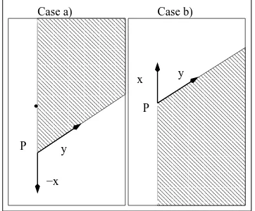
λ2),|λ1|2− |λ2|2), y = (Re(z),Im(z), λ2z+zλ2). We sketchSH+(X) in Figure 5.1 as subsets of the plane E = {P +αx+βy : α, β ∈ R}, for the cases a) ε = 1 and
b)ε=−1, assuming thatxandyare linearly independent. Note that in case a) only one point on the half lineαx, is an element ofSH+(X), while in case b) the whole half line−αxis excluded fromSH+(X).
000000
000000
000000
000000
000000
000000
000000
000000
000000
111111
111111
111111
111111
111111
111111
111111
111111
111111
000
000
111
111
000000
000000
000000
000000
000000
000000
000000
000000
000000
000000
000000
111111
111111
111111
111111
111111
111111
111111
111111
111111
111111
111111
000
000
111
111
0
0
0
0
0
0
0
1
1
1
1
1
1
1
0
0
0
1
1
1
Case a) Case b)
0
1
P y
−x
x y
[image:19.595.202.383.334.484.2]P
Fig. 5.1.Shells of3×3H-normal matrices of type 3 Type 4:
X=
λ z r
0 λ z
0 0 λ
, H =ε
0 0 1 0 1 0 1 0 0
, ε=±1,
where λ, z ∈ C, |z|= 1, 0 ≤argz < π, and r ∈R. By Theorem 5.4, SH+(X) is the
union of an open half plane and a singleton on its boundary. We describeSH+(X) in more detail. Letv= (v1, v2, v3)T ∈C3. Then
v∗Hv=v
3v1+v2v2+v1v3,
v∗HXv=λ(v
3v1+v2v2+v1v3) +z(v3v2+v2v3) +rv3v3,
have to requireα= 0 and|v2|= 1. Thus, the shell ofX has the form
SH+(X) =
P+αx+βy : (α, β)∈R×R+∪ {(0,0)},
where
P =Re(λ),−Im(λ), λλ, x=Re(z),−Im(z), λz+λz, y=r,0, rλ+rλ+ 1.
(Note thatxandyare linearly independent for all possible values ofr∈Randz∈C
with|z|= 1.)
Type 5:
X =
λ 1 ir
0 λ 1 0 0 λ
, H =ε
0 0 1 0 1 0 1 0 0
, ε=±1,
whereλ∈Candr∈R. By Theorem 5.4,S+
H(X) is the union of an open half plane and the singleton on its boundary.
Now we turn to the case when H is singular. By Lemma 2.2, we need only to consider three different cases:
1)H =
1 0 0 0 0 0 0 0 0
, 2)H=
1 0 0 0 1 0 0 0 0
, 3)H =
1 0 0 0 −1 0 0 0 0
.
The first two cases are reduced to shells of 1×1 and 2×2 matrices by Theorem 2.3. Thus, we consider the third case only.
Case 3: Let H1 =
1 0 0 −1
. It follows from the definition that A ∈ C3×3 is
H–normal if and only if it is of the form
A=
A1 dc
∗ ∗
,
(5.6)
whereA1∈C2×2 isH1–normal, and moreover,
|c|=|d| and A∗
1H1
c d
= 0.
(5.7)
Ifc=d= 0, then
HA=
H1A1 0
0 0
, A∗HA=
A∗
1H1A1 0
0 0
and therefore
SinceA1 is a 2×2 H1-normal matrix, it follows from the analysis in Section 5 that
SH+(A) is a line or a half line (open or closed). In particular we have these kinds of shells if detA1= 0, since then we have by the second relation in (5.7) thatc=d= 0. Now let detA1 = 0 and |c| = |d| = 0. Setting δ = d/c(note that by the first relation in (5.7),|δ|= 1) we conclude from the second relation in (5.7) that
A1=
δα δβ
α β
(5.8)
for someα, β∈C. Therefore,
A∗
1H1A1= 0. (5.9)
By (5.6), (5.7), and (5.9),
HA=
H1A1 c
−d
∗ ∗
, A∗HA=
A∗
1H1A1 0
0 0
= 0,
and therefore, upon settingx= (x1, x2, x3)T ∈C3,
S+ H(A)
=
x1 −x2 A1
x1
x2
+c x1 x2
1
−δ
x3, 0
: |x1|2− |x2|2= 1
.
Sincex1−x2δ= 0 for some choice ofx1 andx2subject to|x1|2− |x2|2= 1 it follows thatSH+(A) is the coordinate xy-plane.
In particular, we obtain the following conclusion from the above discussion. Theorem 5.7. Let A be an n×n H-normal matrix, where n ≤ 3. Then the
shellS+
H(A)is a subset of a line ifn= 2, and a subset of a p lane ifn= 3. Moreover,
SH+(A)is convex, and its closure is a polyhedral set.
Thus, Conjecture 5.1 holds true forH-normal matrices of sizes less than 4.
5.4. The case H hasonly one positive eigenvalue. In this subsection, we will prove Conjecture 5.1 for the case thatH is an invertible Hermitian matrix with only one positive eigenvalue. First, let us focus on the blocks of type 5 of Theorem 5.2. These matrices have been extensively used in [15] as a counter example for many statements onH-normal matrices that are true for the case thatHis positive definite. However, we next show that Conjecture 5.1 still holds true.
Proposition 5.8. Let λ∈C,0< φ≤π
2, and
X =
λ cos(φ) sin(φ) 0
0 λ 0 1
0 0 λ 0
0 0 0 λ
, H =ε
0 0 0 1 0 1 0 0 0 0 1 0 1 0 0 0
, ε=±1.
Proof. Using Proposition 2.1(b), we assumeλ= 0. Letv= (v1, v2, v3, v4)T ∈C4 such thatv∗Hv= 1 and let be α, β, γ, δ, η∈R,η≥0 such that
v4v2=α+iβ, v4v3=γ+iδ, v4v4=η.
(5.1)
Note that, on the other hand, for any choice of α, β, γ, δ, η∈R, η >0, there exists a
vectorv ∈C4 such that (5.1) and v4v1+v2v2+v3v3+v1v4 =ε hold, for example,
take
v4=√η, v2=
α+iβ
v4
, v3=
γ+iδ
v4
, v1=
ε− |v2|2− |v3|2 2v4
.
In the case η = 0, we must have v4 = 0 and therefore, such a v ∈ C4 exists if and only ifα=β=γ=δ= 0. A simple computation shows that
v∗HXv=v
4v2cos(φ) +v4v3sin(φ) +v2v4= (α+iβ) cos(φ) + (γ+iδ) sin(φ) +α−iβ,
v∗X∗HXv=v4v4=η.
Thus, setting x1 = (cos(φ) + 1, 0, 0), x2 = (0, cos(φ)−1, 0), x3 = (sin(φ), 0, 0),
x4 = (0, sin(φ), 0), and x5 = (0, 0, 1), and noting that x1 and x3 (x2 and x4, respectively) are linearly dependent, we obtain that
SH+(X) =
α1x1+α2x2+α3x5 : (α1, α2, α3)∈(R×R×R+)∪ {(0,0,0)}
.
Clearly this set is convex and its closure is polyhedral.
For the proof of the main result in this subsection, we will need the following observation.
Lemma 5.9. Let H ∈Cn×n be Hermitian, X ∈Cn×n, and v ∈Cn. If v∗Hv=
α >0, thenv˜:= √1αv satisfiesv˜∗H˜v= 1and
v∗HXv=αv˜∗HXv,˜ v∗X∗HXv=αv˜∗X∗HX˜v.
Consequently, for α >0, we have
(v∗HXv, v∗X∗HXv) : v∈Cn
, v∗Hv=α=αS+
H(X).
Theorem 5.10. Let H be invertible Hermitian and letH have only one positive
eigenvalue. Then the shellS+
H(X)of anH-normal matrixX is convex and its closure
is a polyhedral set.
Proof. Without loss of generality, we may assume thatX andH are in the form of Theorem 5.2. IfX andH are one of the blocks of type 1–5, then the result follows from our discussion in the previous subsections or from Proposition 5.8. Hence, let us assume that X = diag (X1, X2) and H = diag (H1,−Im) are such that X2 ∈
type 1–5 of Theorem 5.2. Letv= (v1, v2)T be partitioned conformably withX and
H. Then
v∗Hv= 1 ⇐⇒ v∗1H1v1= 1 +v2∗v2. Thus, we obtain that the shellSH+(X) ofX is the set
SH+(X)
=(v∗HXv, v∗X∗HXv) : v∗Hv= 1
=(v∗
1H1X1v1, v1∗X1∗H1X1v1)−(v2∗X2v2, v∗2X2∗X2v2) : v∗Hv= 1, v=
v1
v2
=
α≥0
(1 +α)SH+
1(X1)−αS + I (X2)
(by Lemma 5.9 withα=v∗
2v2).
Using the results in the previous subsections and Proposition 5.8, we obtain that
SH+1(X1) consists of all the points of the form
X0+α1X1+α2X2+α3X3,
whereXi∈R1×3 (i= 0,1,2,3) are fixed, and (α1, α2, α3)∈ M. Here,Mstands for one of the sets{0}×{0}×{0},R×{0}×{0},R+×{0}×{0}, (R×R+×{0})∪{0,0,0},
or (R×R×R+)∪ {0,0,0}. Moreover, we know thatSI+(X2) is a polyhedron, i.e., it
has the form
SI+(X2) =
β1Y1+. . .+βlYl : βi≥0,
l
i=1
βi= 1
.
Hence,SH+(X) consists of all the points of the form
(1 +α)(X0+α1X1+α2X2+α3X3)−α(β1Y1+. . .+βlYl)
=X0+αα1X1+αα2X2+αα3X3+αβ1Z1+. . .+αβlZl,
where α ≥ 0, (α1, α2, α3) ∈ M, Zi = X0− Yi, βi ≥0, i = 1, . . . , l, li=1βi = 1. Consequently,
SH+(X) =
X0+ ˜α1X1+ ˜α2X2+ ˜α3X3+ ˜β1Z1+. . .+ ˜βlZl : (˜α1,α˜2,α˜3)∈ M,β˜i≥0
.
Clearly, this set is convex. The closure ofS+
H(X) is finitely generated (in the termi-nology of [16]) and hence polyhedral ([16, Theorem 19.1]).
6. Infinite dimensional case. The concept of the shell makes sense also for operators in infinite dimensional Hilbert spaces. Thus, letHbe an infinite dimensional complex Hilbert space with the inner productx, y, and letH be a fixed bounded selfadjoint operator onHwhich is not negative semidefinite. For a (linear bounded) operatorAonHdefine
where [x, y]H =Hx, y,x, y ∈ H. Many results of Sections 2 and 3 admit straight-forward generalization to the infinite dimensional case, or parallel results for this case can be developed. We note thatH-normal operators are defined (via (2.5)) only if
H has a Moore-Penrose inverse, and therefore this hypothesis is implicitly assumed each time aH-normal operator appears. As it is well-known,H has a Moore-Penrose inverse if and only if the range ofH is a closed subspace. Thus, the results of Section 2 (except Proposition 2.5) go over to the infinite dimensional case essentially without changes.
Next, consider the geometric properties of shells. Theorem 3.3 is obviously valid also in the infinite dimensional case. To prove Theorem 3.5(a) in this case, assume first that S+
H(A) is a singleton. Fix v ∈ H such that [v, v]H = 1. Then for every
u∈ H and for every α∈Csufficiently close to zero, [v+αu, v+αu]H >0. Scaling
v+αuappropriately, and using the property thatS+
H(A) is a singleton, we obtain
HA(v+αu), v+αu=H(v+αu), v+αu HAv, v.
Lettingαbe real, it follows thatHAu, u=Hu, u HAv, vby equating coefficients ofα2. Sinceu
∈ His arbitrary, we must haveHA=cH,c∈C, as required.
For Theorem 3.5(b), first observe that if the operators H,HA+A∗H, i(HA−
A∗H), A∗HA span a two dimensional real subspace, then S+
H(A) is easily seen to be a subspace of a line. Conversely, assume SH+(A) ⊆ {r+tq : t ∈ R} for some vectors r, q ∈ R1×3. Applying transformations of Proposition 2.1, we may without
loss of generality assume that two out of the three components ofqare zeros. Say for instance, the first and the third components ofqare zero (in other cases, the proof is analogous). Then withu,v, andαas in the preceding paragraph, we have
(HA+A∗H)(v+αu), v+αu=H(v+αu), v+αu (HA+A∗H)v, v,
HA(v+αu), A(v+αu)=H(v+αu), v+αu HAv, Av.
Again, equating the coefficients of α2 in both sides of each of these equalities, we obtain thatHA+A∗H andA∗HAare scalar multiples ofH, concluding the proof.
Finally, consider boundedness. Recall the definition (introduced in [14]) of the
numerical rangewith respect to the indefinite inner product induced byH:
WH+(A) ={[Av, v]H :v∈ H,[v, v]H= 1}.
Theorem 6.1. Let H be a selfadjoint operator onH, not negative semidefinite.
Then the following statements are equivalent for an operator AonH:
(1) The numerical range WH+(A)is bounded. (2) The shell S+
H(A)is bounded.
(3) EITHERH is indefinite andHA=αH for someα∈C, OR the properties
(i) and(ii)below are satisfied: (i)H is positive semidefinite;(ii) the linear setRange (√H)isA∗-invariant, where√H is the positive semidefinite square root ofH.
7. A Maple program. Here we include a Maple program which displays a portion of the shellSH+(A) that helped us to formulate and check conjectures at the early stage of our project.
The procedures are limited to parameterization of a vector based on variablesr
andα. Inplotshell2one can specifyv, however, the ranges ofrandαare fixed to
r=−10· ·10 and α=−2π· ·2π, butX (and correspondinglyv) may have arbitrary
dimensions. Inplotshellthe vectorv is fixed tov=
reiα
i
, but one can change
the ranges ofrandα.
> restart;with(plots):with(linalg): Warning, new definition for norm Warning, new definition for trace
> # This procedure, takes a H for the hermitian > # matrix that defines the inner
> # product, an X for the matrix, and a V given > # by the user ‘a‘ represents the magnitude > # of v since we only want [v,v]=1 b is the > # numerical range not divided by the norm of v > # x1,x2 are the real and imaginary components of the > # numerical range x3 is the second component [Xv,Xv] > # This plots x1,x2,x3 parameterized by a
> # vector that depends on a phase alpha and a magnitude r >
> plotshell2 := proc (H, X, V) > local a, b, x1, x2, x3;
> a:=simplify(multiply(htranspose(V),H,V)); > b:=simplify(multiply(htranspose(V),H,X,V)); > x1:=simplify(Re(b[1,1])/a[1,1]);
> x2:=simplify(Im(b[1,1])/a[1,1]);
> x3:=simplify(multiply(htranspose(V),htranspose(X),H,X,V))[1,1] /a[1,1];
> plot3d([x1, x2, x3],alpha = -2*Pi..2*Pi,r = -10..10); end; >
> # This is a similar procedure only the v is fixed, > # but you can change the parameterization values or r > # and alpha by calling it with an rlow rhigh
> # and alphalow and alphahigh >
> plotshell := proc(H, X, rlow,rhigh,alphalow,alphahigh) > local a, b, x1, x2, x3,V;
> assume(r,real,alpha,real):
> x2:=simplify(Im(b[1,1])/a[1,1]);
> x3:=simplify(multiply(htranspose(V),htranspose(X),H,X,V))[1,1] /a[1,1];
> plot3d([x1, x2, x3],alpha = alphalow .. alphahigh,r= rlow .. rhigh) end;
REFERENCES
[1] P. Binding and C. K. Li. Joint ranges of Hermitian matrices and simultaneous diagonalization.
Linear Algebra Appl., 151:157–168, 1991.
[2] M.-T. Chien and H. Nakazato. Davis-Wielandt shell andq-numerical range. Linear Algebra Appl., 340:15–31, 2002.
[3] C. Davis. The shell of a Hilbert-space operator. Acta Sci. Math.(Szeged), 29:69–86, 1968. [4] C. Davis. The shell of a Hilbert-space operator. II.Acta Sci. Math.(Szeged), 31:301–318, 1970. [5] R. G. Douglas. On majorization, factorization, and range inclusion of operators in Hilbert
space.Proc. Amer. Math. Soc., 17:413–415, 1966.
[6] I. Gohberg and B. Reichstein. On classification of normal matrices in an indefinite scalar product.Integral Equations Operator Theory, 13:364–394, 1990.
[7] I. Gohberg and B. Reichstein. On H-unitary and block-Toeplitz H-normal operators. Linear and Multilinear Algebra, 30:17–48, 1991.
[8] I. Gohberg and B. Reichstein. Classification of block-Toeplitz H-normal operators.Linear and Multilinear Algebra, 34:213–245, 1993.
[9] R. A. Horn and C. R. Johnson.Topics in Matrix Analysis.Cambridge University Press, Cam-bridge, 1991.
[10] C. K. Li and H. Nakazato. Some results on the q-numerical range. Linear and Multilinear Algebra, 43: 385–409, 1998.
[11] C. K. Li and L. Rodman. Remarks on numerical ranges of operators in spaces with an indefinite metric.Proc. Amer. Math. Soc., 126:973–982, 1998.
[12] C. K. Li and L. Rodman. Shapes and computer generation of numerical ranges of Krein space operators. Electronic Linear Algebra, 3:31–47, 1998.
[13] C. K. Li and L. Rodman. H–joint numerical ranges, to appear inBull. of Australian Math. Soc.(Preprint available at http://www.resnet.wm.edu/ cklixx/jhw.pdf).
[14] C. K. Li, N. K. Tsing, and F. Uhlig. Numerical ranges of an operator on an indefinite inner product space.Electronic Linear Algebra, 1:1–17, 1996.
[15] C. Mehl and L. Rodman. Classes of matrices in indefinite inner products.Linear Algebra Appl., 336:71–98, 2001.